Previous articles in this series:
- 1. Motivations and Methods
- 2. Obtaining OpenStreetMap data
- 3. Manipulating geodata with GeoPandas
- 4. Cleaning text data with fuzzywuzzy
- 5. Building a street name classifier with scikit-learn
In the last article, we built a baseline classifier for street names. The results were a bit disappointing at 55% accuracy. In this article, we’ll add more features, and streamline the code with scikit-learn’s Pipeline and FeatureUnion classes.
I learned a lot about Pipelines and FeatureUnions from Zac Stewart’s article on the subject, which I recommend.
Adding features
There’s a great paper called A few useful things to know about machine learning by Pedros Domingos, one of the most prominent researchers in the field, in which he says:
At the end of the day, some machine learning projects succeed and some fail. What makes the difference? Easily the most important factor is the features used…This is typically where most of the effort in a machine learning project goes.
So far I’d only used n-grams. But there were other sources of information I wasn’t using. Some ideas I had for more features were:
- Number of words in name
- More words: likely to be Chinese (e.g. “Ang Mo Kio Avenue 1”)
- Average word length
- Shorter: likely to be Chinese (e.g. “Ang Mo Kio”)
- Longer: likely to be British or Indian (e.g. “Kadayanallur Street”)
- Are all the words in the dictionary?
- Yes: likely to be Generic (e.g. “Cashew Road”). Funny exception: Boon Lay Way (Chinese)
- Is the “road tag” Malay?
- Yes: likely Malay (e.g. “Jalan Bukit Merah”, “Lorong Penchalak”, vs “Upper Thomson Road”, “Ang Mo Kio Avenue 1”)
How to incorporate these into the previous code? Let’s look at the code we needed to create the n-gram feature matrix:
from sklearn.feature_extraction.text import CountVectorizer
from sklearn.svm import LinearSVC

# build the feature matrices
ngram_counter = CountVectorizer(ngram_range=(1, 4), analyzer='char')
X_train = ngram_counter.fit_transform(data_train)
X_test  = ngram_counter.transform(data_test)

# train the classifier
classifier = LinearSVC()
model = classifier.fit(X_train, y_train)

# test the classifier
y_test = model.predict(X_test)
To add the new features, what we’re looking at is:
- Writing functions that produce a feature vector for each feature
- Repeating the
fit_transformandfitlines for each feature - Adding two lines of code where we combine the resultant
numpymatrices into a one giant training feature matrix and one testing feature matrix
This may not seem like a huge deal, but it is pretty repetitive, opening ourselves up to the possibility of errors, for example calling fit_transform on the testing data rather than just transform.
Fortunately, scikit-learn gives us a better way: Pipelines.
Pipelines
Another way to think about the code above is to imagine a pipeline that takes in our input data, puts it through a first transformer – the n-gram counter – then through another transformer – the SVC classifier – to produce a trained model, which we can then use for prediction.
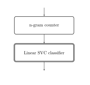
This is precisely what the Pipeline class in scikit-learn does:
from sklearn.feature_extraction.text import CountVectorizer
from sklearn.svm import LinearSVC

# build the pipeline
ppl = Pipeline([
              ('ngram', CountVectorizer(ngram_range=(1, 4), analyzer='char')),
              ('clf',   LinearSVC())
      ])

# train the classifier
model = ppl.fit(data_train)

# test the classifier
y_test = model.predict(data_test)
Notice that this time, we’re operating on data_train and data_test,
i.e. just the lists of road names. We didn’t have to manually create a separate
feature matrix for training and testing – the pipeline takes care of that.
Creating a new transformer
Now we want to add a new feature – average word length. There’s no built-in
feature extractor like CountVectorizer for this, so we’ll have to write our
own transformer. Here’s the code to do that. This time, instead of a list of
names, we’re going to start passing in a Pandas dataframe, which has a column
for the street name and another column for the “road tag”
(Street, Avenue, Jalan, etc).
from sklearn.base import BaseEstimator, TransformerMixin

class AverageWordLengthExtractor(BaseEstimator, TransformerMixin):
    """Takes in dataframe, extracts road name column, outputs average word length"""

    def __init__(self):
        pass

    def average_word_length(self, name):
        """Helper code to compute average word length of a name"""
        return np.mean([len(word) for word in name.split()])

    def transform(self, df, y=None):
        """The workhorse of this feature extractor"""
        return df['road_name'].apply(self.average_word_length)

    def fit(self, df, y=None):
        """Returns `self` unless something different happens in train and test"""
        return self
Unless you’re doing something more complicated where something different happens in the training and testing phase (like when extracting n-grams), this is the general pattern for a transformer:
from sklearn.base import BaseEstimator, TransformerMixin

class SampleExtractor(BaseEstimator, TransformerMixin):

    def __init__(self, vars):
        self.vars = vars  # e.g. pass in a column name to extract

    def transform(self, X, y=None):
        return do_something_to(X, self.vars)  # where the actual feature extraction happens

    def fit(self, X, y=None):
        return self  # generally does nothing
Now that we’ve created our transformer, it’s time to add it into the pipeline.
FeatureUnions
We have a slight problem: we only know how to add transformers in series, but what we need to do is to add our average word length transformer in parallel with the n-gram extractor. Like this:
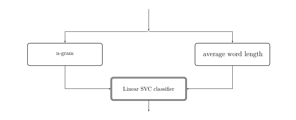
For this, there is scikit-learn’s FeatureUnion class.
from sklearn.pipeline import Pipeline, FeatureUnion

pipeline = Pipeline([
    ('feats', FeatureUnion([
        ('ngram', ngram_count_pipeline), # can pass in either a pipeline
        ('ave', AverageWordLengthExtractor()) # or a transformer
    ])),
    ('clf', LinearSVC())  # classifier
])
Notice that the first item in the FeatureUnion is ngram_count_pipeline.
This is just a Pipeline created out of a column-extracting transformer,
and CountVectorizer (the column extractor is necessary
now that we’re operating on a Pandas dataframe
rather than directly sending the list of road names through the pipeline).
That’s perfectly okay: a pipeline is itself just a giant transformer, and is treated as such. That makes it easy to write complex pipelines by building smaller pieces and then putting them together in the end.
Conclusion
So what happened after adding in all these new features? Accuracy went up to 65%, so that was a decent result. Note that using Pipelines and FeatureUnions did not in itself contribute to the performance. They’re just another way of organising your code for readability, reusability and easier experimentation.
If you’re looking to do hyperparameter tuning (which I won’t explain here), pipelines make that easy, as below:
from sklearn.grid_search import GridSearchCV

pg = {'clf__C': [0.1, 1, 10, 100]}

grid = GridSearchCV(pipeline, param_grid=pg, cv=5)
grid.fit(data_train, y_train)

grid.best_params_
# {'clf__C': 0.1}

grid.best_score_
# 0.702290076336
Ultimately, after adding in more features, adding more data, and doing hyperparameter tuning, I had about 75-80% accuracy, which was good enough for me. I only had to hand-correct 20-25% of the roads, which didn’t seem too daunting. I was ready to make my map. That’s what we’ll do in the next article.