Previous articles in this series:
- 1. Motivations and Methods
- 2. Obtaining OpenStreetMap data
- 3. Manipulating geodata with GeoPandas
- 4. Cleaning text data with fuzzywuzzy
In this fifth article, we’ll look at how to build a classifier, classifying street names by linguistic origin, using scikit-learn.
Step 1: pick a classification schema
Often, when building a classifier, you have a pretty good idea of what you want to classify your items as: as spam or ham, as one of these six species of iris, etc. For me, it was a bit less clear. There’s the obvious “big four” ethnicities of Singapore: Chinese, Malay, Indian, and Other. But there are dialects (really, languages) of Chinese, ditto with Indian, and how does one split up “Other”?
In the end, after some data exploration and some thought about what I wanted to see on the map, I went with:
- Chinese (all dialects including Cantonese, Hokkien, Mandarin, etc)
- Malay
- Indian (all languages of the subcontinent)
- British
- Generic (Race Course Road, Sunrise Place)
- Other (generally other languages).
Six seemed about right: reducing the number of categories would make for meaningless clusters; increasing the number of categories would result in an indecipherable map.
So that’s Step 1 done.
Step 2: create some training and testing data
To train the classifier, we need to give it some examples: MacPherson is a British name, Keng Lee is a Chinese name. So I went ahead and hand-coded about 10% of the dataset (200 street names).
This was pretty tricky because even when you’ve picked a classification schema, it may not be obvious how to categorise individual items into those categories. For example, “Florence Road” is named after a Chinese woman, Florence Yeo. But the street name sounds pretty English, or perhaps it should be under Other since it’s derived from the Latin. So I came up with some guidelines for myself on how to categorise them. (“Florence Road” was classified Chinese, in the end – pretty much impossible for the classifier to get it right, but that’s how I wanted it in the map.)
Once we have this data, we need to divide it into a train set and a test set. scikit-learn gives us a function, train_test_split, to do this easily:
from sklearn.cross_validation import train_test_split

data_train, data_test, y_train, y_true = \
    train_test_split(df['road_name'], df['classification'], test_size=0.2)
Here, data_train and data_test are the street names, while y_train and y_test are the classifications into British, Chinese, Malay, etc. And we did an 80-20 split, which is quite normal.
Step 3: Choose features
Classifiers don’t really work on strings like street names. They work on numbers, either integers or reals. So we need to find a way to convert our street names to something numeric that the classifier can sink its teeth into.
One really common text feature is n-gram counts. These are overlapping substrings of length n. To make this concrete, take the street name “(Jalan) Malu-Malu”, focusing just on the “Malu-Malu” part.
There are five 1-grams, or unigrams: “m” (count: 2), “a” (2), “l” (2), “u” (2), and “-“ (1).
The 2-grams, or bigrams, are “ma” (count: 2), “al” (2, notice the overlap!), “lu” (2), and so on. In addition, we often put a special character at the beginning and end, let’s call it “#”, so there’s also “#m” (count: 1), “u#” (count: 1).
The 3-grams, or trigrams, are “##m” (count: 1), “#ma” (1), “mal” (2), etc. You get the picture.
Why pick n-grams? Basically, we need features that are simple to compute, and discriminate between the various categories. Here are the n-gram counts for a 2-gram (or bigram), “ck”.
| British | Chinese | Malay | Indian |
|---|---|---|---|
| 23 | 17 | 0 | 0 |
| Alnwick | Boon Teck | ||
| Berwick | Hock Chye | ||
| Brickson | Kheam Hock | ||
| … | … |
So, when the classifier sees “ck” in a street name, it can say with confidence that it’s not Malay or Indian. Basically, n-grams are a quick and easy way to capture the orthotactic patterns of a language: what letter combinations are likely to occur?
I promised that computing these would be easy. That’s because scikit-learn has our back for computing these n-gram counts, in the form of the CountVectorizer class. Here’s how to use it:
from sklearn.feature_extraction.text import CountVectorizer

# compute n-grams of size 1 through 4
ngram_counter = CountVectorizer(ngram_range=(1, 4), analyzer='char')

X_train = ngram_counter.fit_transform(data_train)
X_test  = ngram_counter.transform(data_test)
This gives us X_train, a numpy array with each row representing a street name,
columns representing the n-grams, and each cell representing the count of the
n-gram in that street name.
Notice that there’s a different function for training, fit_transform,
than testing, where it’s just transform. The reason for this is that
we need to have exact same features in training as well as in testing.
There’s no point having a new n-gram in the test set, since
the classifier will not have any information about how well it correlates
with the various labels.
Step 4: Select a classifier
There are a bunch of classification algorithms included in scikit-learn.
They all share the same API, so it’s really easy to swap them around. But
we need to know where to start. The scikit-learn folks helpfully provide
this diagram to pick a classification tool.

If you follow the steps, we wind up at Linear SVC, so that’s what we’ll use.
Step 5: Train the classifier
First, the code:
from sklearn.svm import LinearSVC

classifier = LinearSVC()

model = classifier.fit(X_train, y_train)
Now, let’s get some intuition for what’s going on.
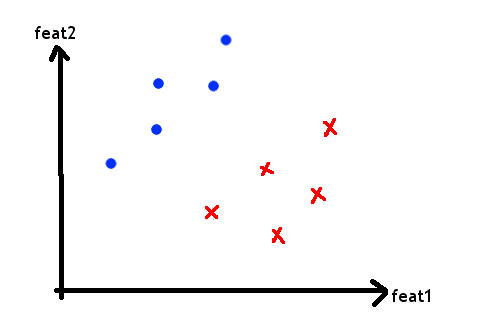
We can think of each of our street names as a point in an n-dimensional feature space. For the purposes of illustration, let’s pretend there are just 2 features, and that it looks like this, with red crosses representing Chinese street names and blue dots representing British street names.
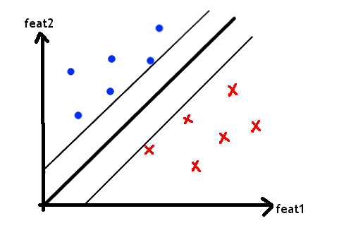
What the Linear SVC classifier does is to draw a line in between the two sets of points as best it can, with as large a margin as possible.

This line is our model.
Now suppose we have two new points that we don’t know the labels of.
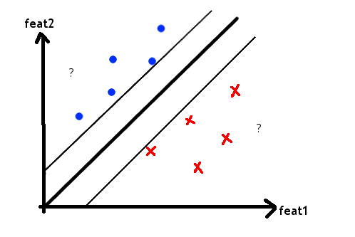
The classifier looks at where they fall with respect to the line, and tells us whether they’re Chinese or British.
Obviously, I’ve simplified a lot of things. In higher-dimensional space, the line becomes a hyperplane. And of course, not all datasets fall so smoothly into separate camps. But the basic intuition is still the same.
Step 6: Test the classifier
At the end of the last step, we had model, a trained classifier object.
We can now use it to classify new data, as was explained above,
and see how correct it is by
comparing it to the actual predictions I hand-coded in Step 2.
y_test = model.predict(X_test)

sklearn.metrics.accuracy_score(y_true, y_test)
# 0.551818181818
scikit-learn has a bunch of metrics built in. Choose the one that best
reflects how you’ll use and assess the classifier. In my case, my workflow
was to use the classifier to predict the labels of streets I had never
hand-coded, and correct the ones that were incorrect, rather than doing
everything from scratch. I wanted to save time by having as few incorrect ones
as possible, so accuracy was the right metric. But if you have different priorities,
other metrics might make more sense.
Improving the classifier
So we wound up with an accuracy of 55%. That sounds like chance, but it isn’t: we had 6 categories, so chance is really 16.6%.
There’s another super-dumb way of classifying things, to pretend that everything is Malay, the most common classification. That would give us 35% accuracy. So we’re 20% above the baseline.
Our likely upper bound is around 90%, because of names like “Florence” where it’s really unclear. We’re 35% away from that, so it should be possible to make things a lot better.
Here are some ideas for improving it:
- Use more data. More training data is always better, but it’s more work.
- Trying other classifiers. We could swap in another classifier for Linear SVC. Might help.
- Adding more features. Yes! There’s a lot of information in the data that’s not reflected by n-grams. We could try that.
- Hyperparameter tuning. We invoked
LinearSVCwith no arguments, but we can pass it hyperparameters that tweak how it works. This is pretty fiddly. Let’s see where we get with the other strategies.
In the next article, I’ll talk about how to easily add more features to our classifier. Till then.