A gentle introduction to deep learning with TensorFlow
Michelle Fullwood
@michelleful
Slides: michelleful.github.io/PyCon2017
Prerequisites
- Knowledge of concepts of supervised ML
- Familiarity with linear and logistic regression
Target
(Deep) Feed-forward neural networks
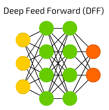
- How they're constructed
- Why they work
- How to train and optimize them
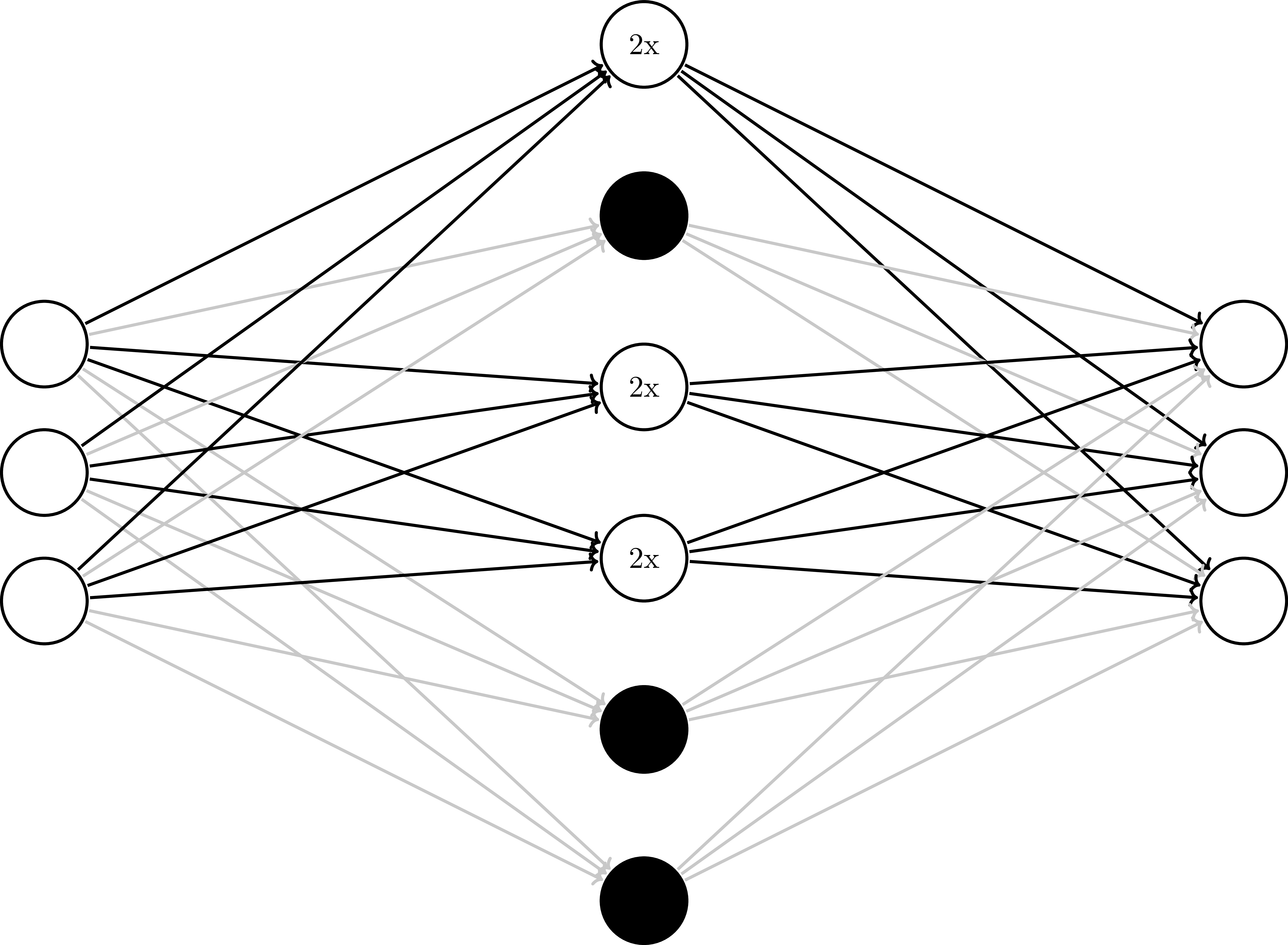
Image source: Fjodor van Veen (2016) Neural Network Zoo
Deep learning learning curve
Deep learning learning curve
Deep learning learning curve
Deep learning learning curve
Deep learning learning curve

|
|
| Traditional machine learning | Deep learning |
TensorFlow
- Popular deep learning toolkit
- From Google Brain, Apache-licensed
- Python API, makes calls to C++ back-end
- Works on CPUs and GPUs
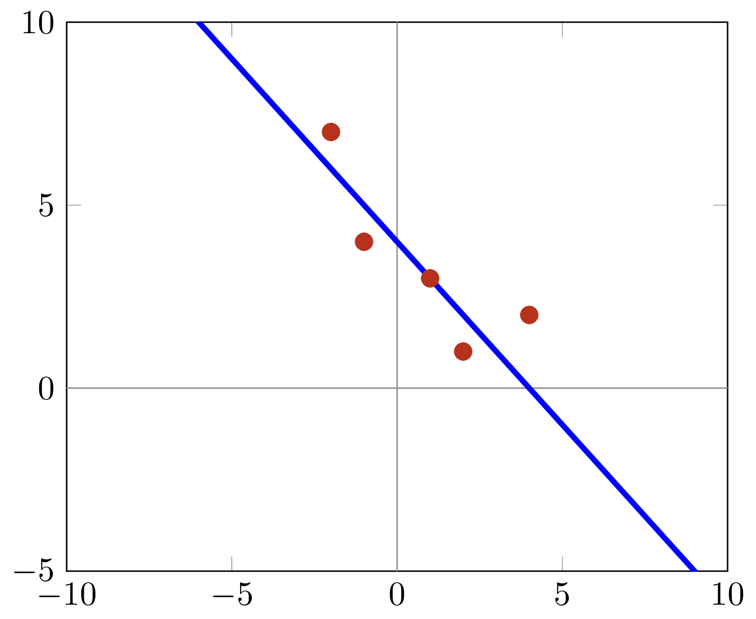
Linear Regression
from scratch
Linear Regression


Inputs

Inputs
X_train = np.array([
    [1250, 350, 3],
    [1700, 900, 6],
    [1400, 600, 3]
])

Y_train = np.array([345000, 580000, 360000])
Model
Multiply each feature by a weight and add them up.
Add an intercept to get our final estimate.
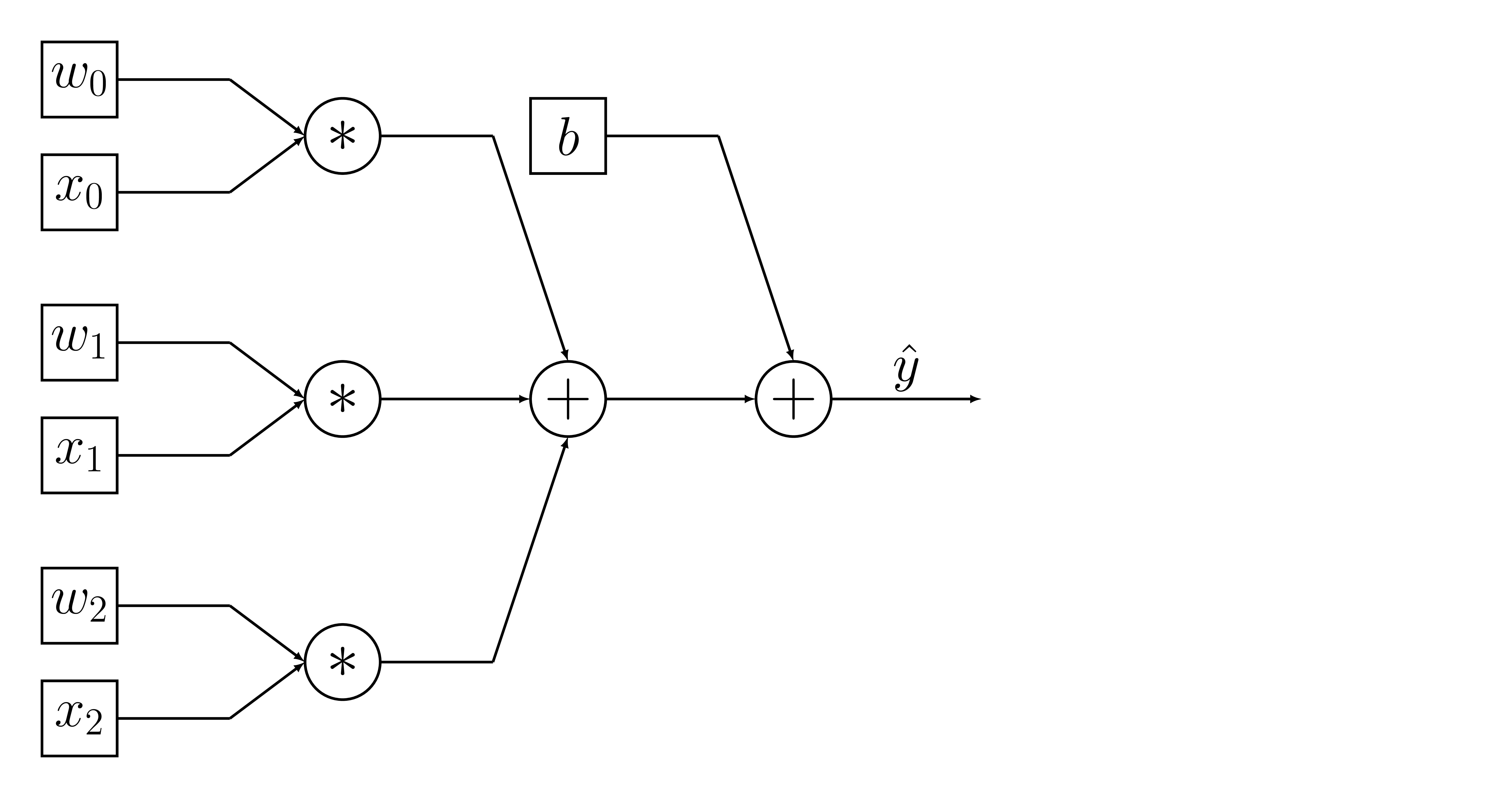
Model
Model - Parameters
weights = np.array([300, -10, -1])
intercept = -26497
Model - Operations
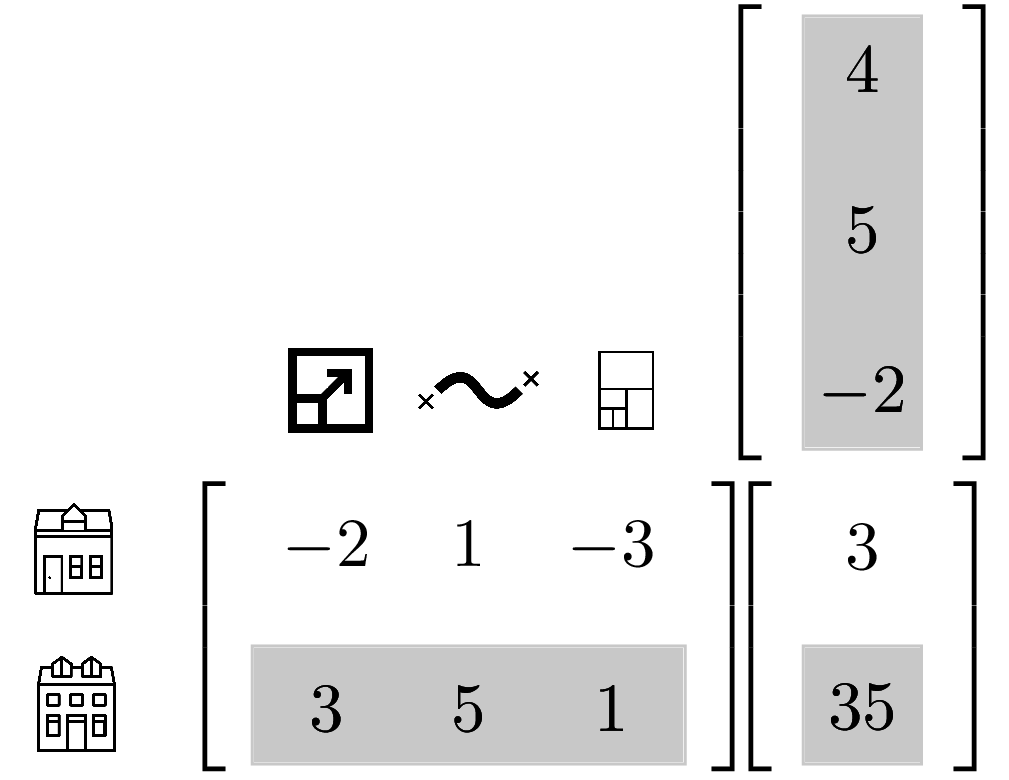
Model - Operations
def model(X, weights, intercept):
    return X.dot(weights) + intercept

Y_hat = model(X_train, weights, intercept)
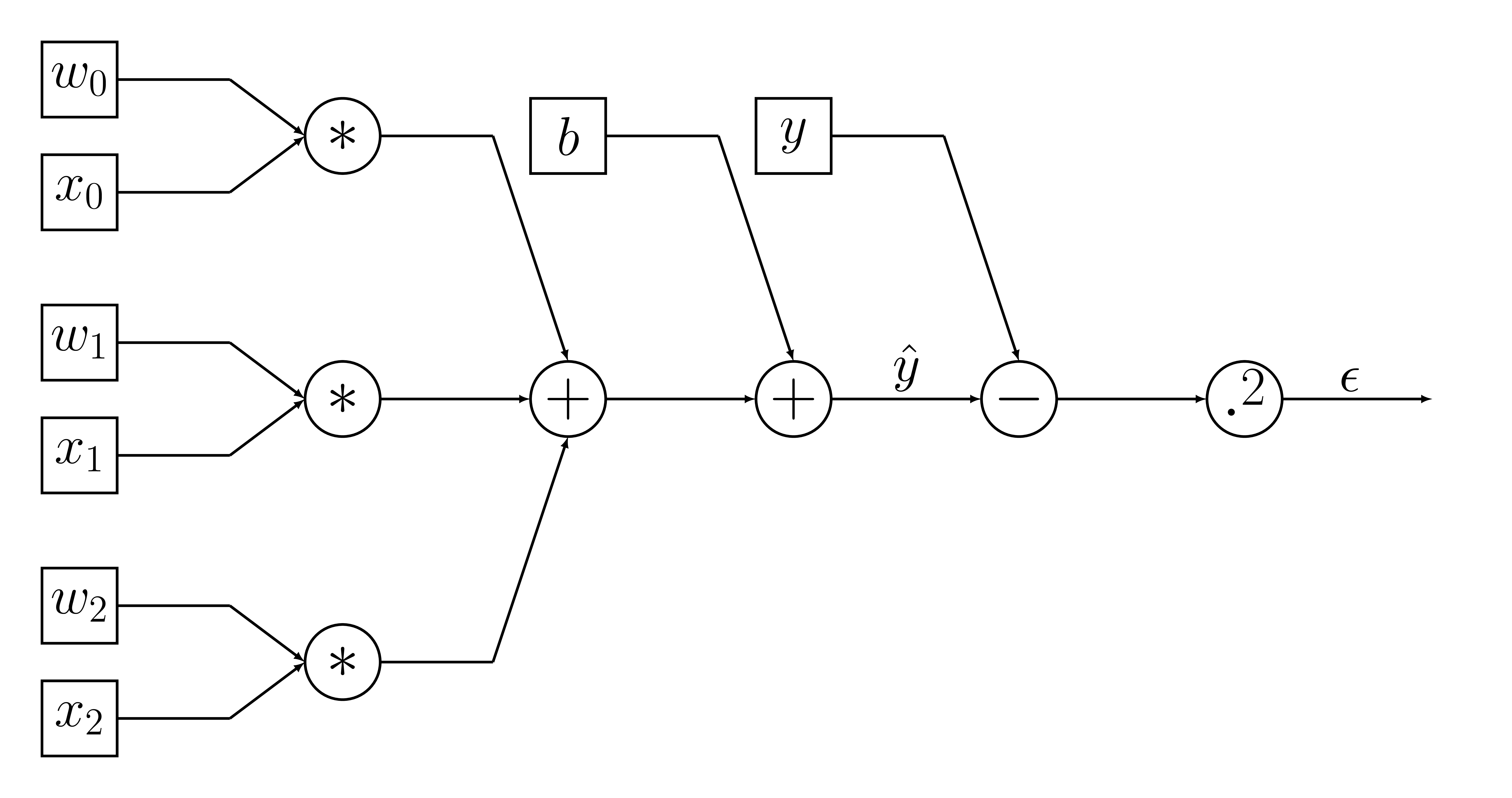
Model - Cost function
Model - Cost function
Model - Cost function
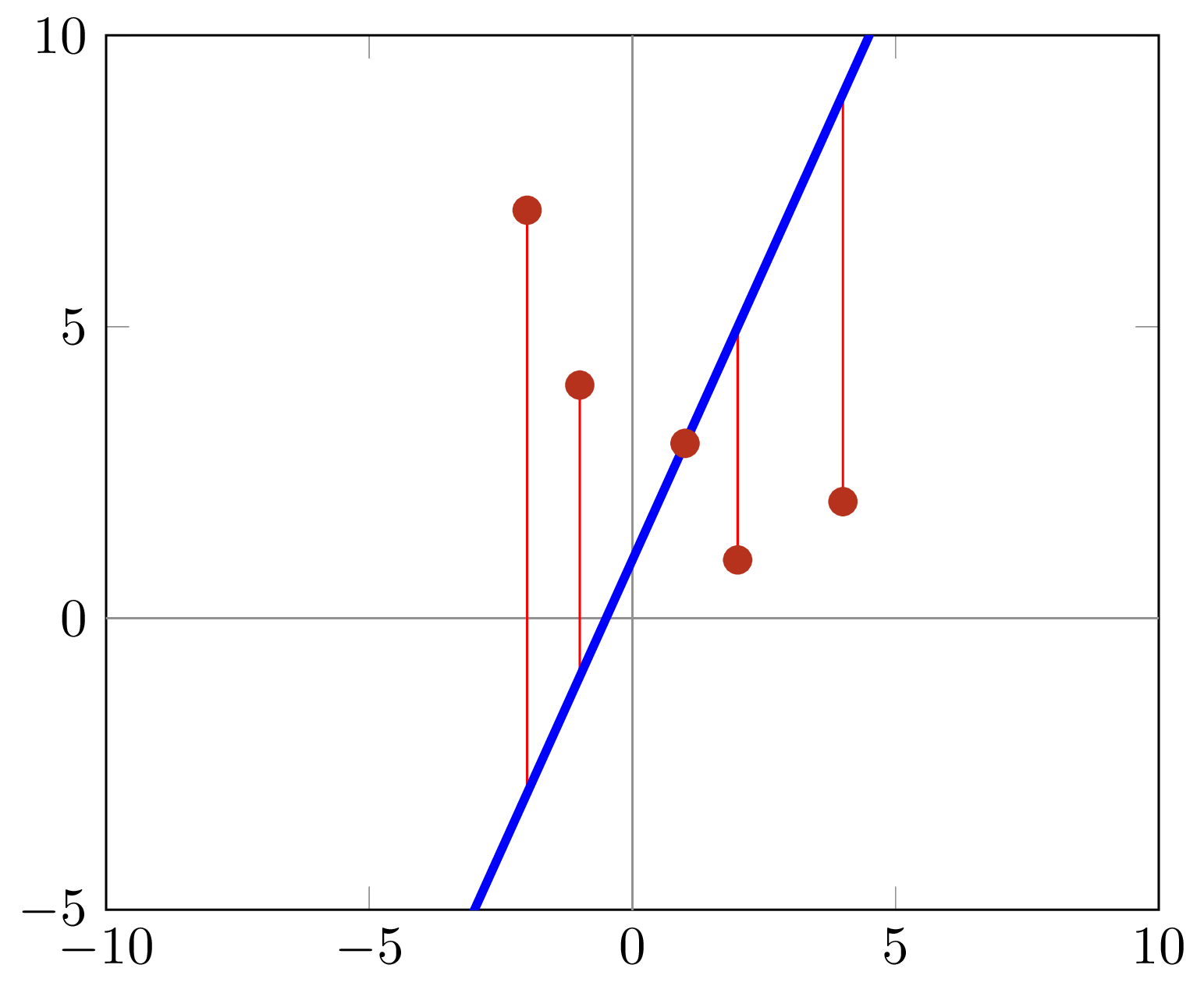
Cost function
def cost(Y_hat, Y):
    return np.sum((Y_hat - Y)**2)
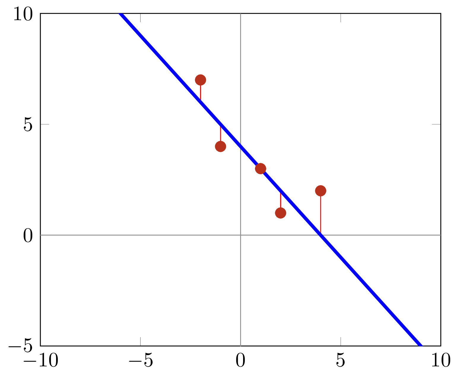
Optimization
Hold X and Y constant.
Adjust parameters to minimize cost.
Optimization
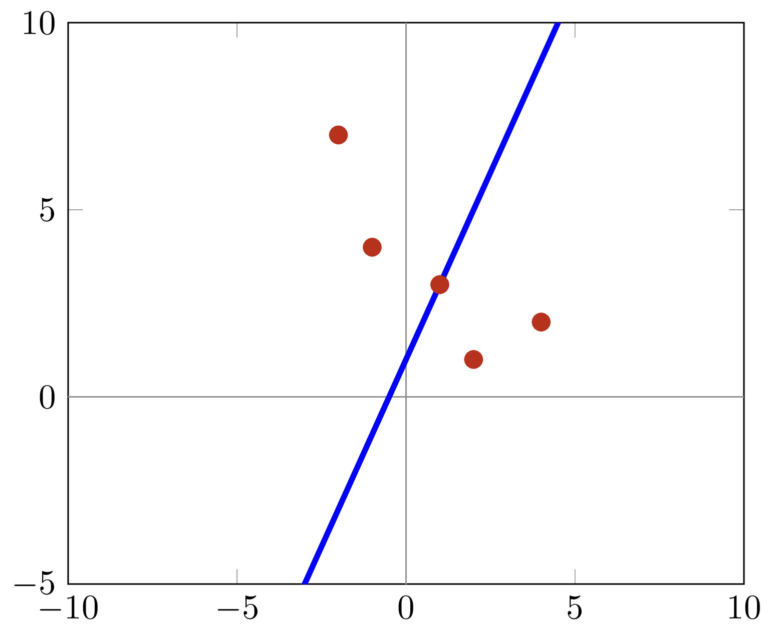
Trial and error

Image source: Wikimedia Commons
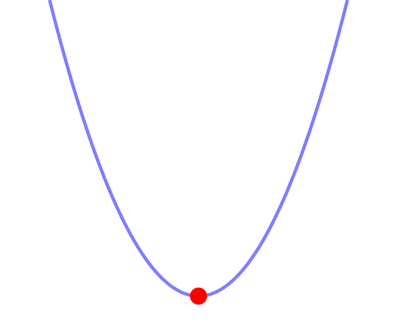
Optimization
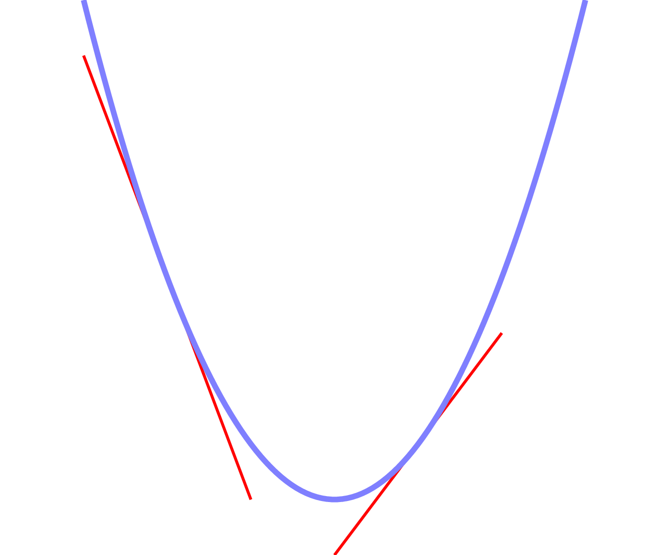
Optimization
Optimization - Gradient Calculation
$$\hat{y} = w_0x_0 + w_1x_1 + w_2x_2 + b$$ $$\epsilon = (y-\hat{y})^2$$
Goal: \(\frac{\partial\epsilon}{\partial w_i}, \frac{\partial\epsilon}{\partial b}\)
Optimization - Gradient Calculation
Chain rule: \(\frac{\partial\epsilon}{\partial w_i} = \frac{d\epsilon}{d\hat{y}}\frac{\partial\hat{y}}{\partial w_i} \)
Optimization - Gradient Calculation
$$\hat{y} = w_0x_0 + w_1x_1 + w_2x_2 + b$$
\(\frac{\partial\hat{y}}{\partial w_0} =\)\( x_0\)
Optimization - Gradient Calculation
$$\epsilon = (y-\hat{y})^2$$
\(\frac{d\epsilon}{d\hat{y}} =\) \(-\)\(2(y-\hat{y})\)
Optimization - Gradient Calculation
\(\frac{\partial\hat{y}}{\partial w_0} = x_0\)
\(\frac{d\epsilon}{d\hat{y}} = -2(y-\hat{y})\)
\(\frac{\partial\epsilon}{\partial w_0} = -2(y-\hat{y})x_0 \)
Optimization - Gradient Calculation
$$\hat{y} = w_0x_0 + w_1x_1 + w_2x_2 + b\cdot1$$
\(\frac{\partial\epsilon}{\partial b} = -2(y-\hat{y})\cdot 1 \)
Optimization - Gradient Calculation
		delta_y = y - y_hat
		gradient_weights = -2 * delta_y * weights
		gradient_intercept = -2 * delta_y * 1
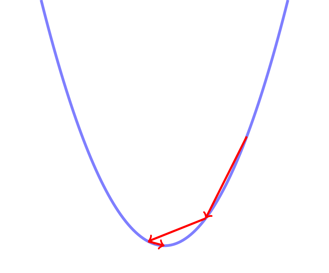
Optimization - Parameter Update
weights = weights - gradient_weights
intercept = intercept - gradient_intercept
Optimization - Overshoot
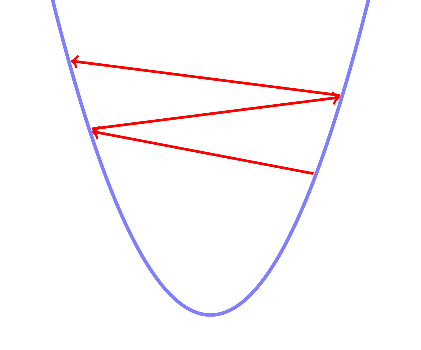
Optimization - Undershoot
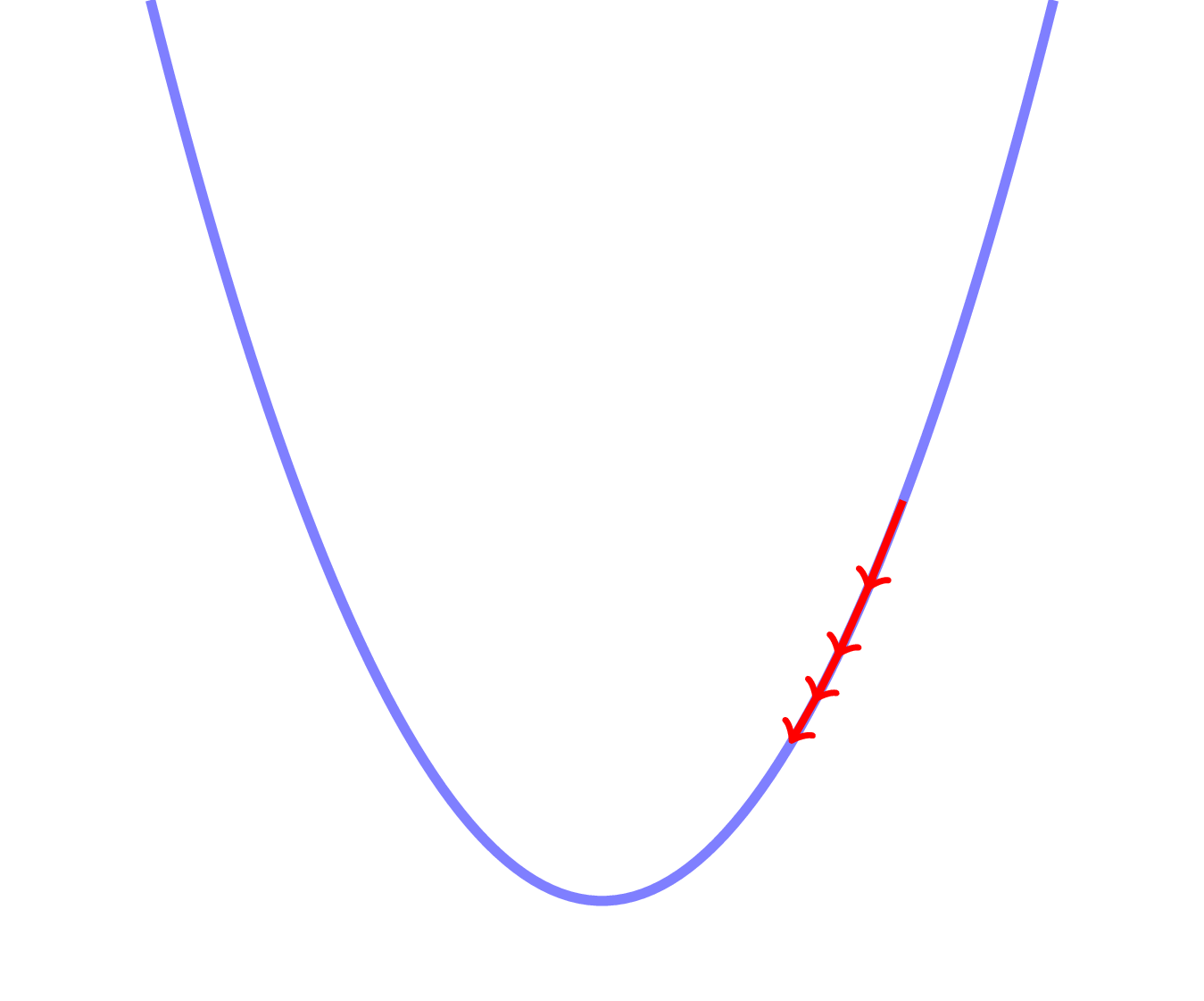
Optimization - Parameter Update
learning_rate = 0.05

weights = weights - \
             learning_rate * gradient_weights
intercept = intercept - \
             learning_rate * gradient_intercept
Training
def training_round(x, y, weights, intercept,
                   alpha=learning_rate):
    # calculate our estimate
    y_hat = model(x, weights, intercept)

    # calculate error
    delta_y = y - y_hat

    # calculate gradients
    gradient_weights = -2 * delta_y * weights
    gradient_intercept = -2 * delta_y

    # update parameters
    weights = weights - alpha * gradient_weights
    intercept = intercept - alpha * gradient_intercept

    return weights, intercept
Training
NUM_EPOCHS = 100

def train(X, Y):
    # initialize parameters
    weights = np.random.randn(3)
    intercept = 0

    # training rounds
    for i in range(NUM_EPOCHS):
        for (x, y) in zip(X, Y):
            weights, intercept = training_round(x, y,
                                 weights, intercept)
Testing
def test(X_test, Y_test, weights, intercept):
    Y_predicted = model(X_test, weights, intercept)
    error = cost(Y_predicted, Y_test)
    return np.sqrt(np.mean(error))

>>> test(X_test, Y_test, final_weights, final_intercept)
6052.79
Surprise!
You've already made
a neural network!
Linear regression =
Simplest neural network

Once more, with TensorFlow
- Inputs
- Model - Parameters
- Model - Operations
- Cost function
- Optimization
- Train
- Test
Inputs → Placeholders
import tensorflow as tf

X = tf.placeholder(tf.float32, [None, 3])
Y = tf.placeholder(tf.float32, [None, 1])
Parameters → Variables
# create tf.Variable(s)
W = tf.get_variable("weights", [3, 1],
       initializer=tf.random_normal_initializer())
b = tf.get_variable("intercept", [1],
       initializer=tf.constant_initializer(0))
Operations
Y_hat = tf.matmul(X, W) + b
Cost function
cost = tf.reduce_mean(tf.square(Y_hat - Y))
Optimization
learning_rate = 0.05
optimizer = tf.train.GradientDescentOptimizer
               (learning_rate).minimize(cost)
Training
with tf.Session() as sess:
    # initialize variables
    sess.run(tf.global_variables_initializer())

    # train
    for _ in range(NUM_EPOCHS):
        for (X_batch, Y_batch) in get_minibatches(
               X_train, Y_train, BATCH_SIZE):
            sess.run(optimizer,
                     feed_dict={
                         X: X_batch,
                         Y: Y_batch
                     })
# Placeholders
X = tf.placeholder(tf.float32, [None, 3])
Y = tf.placeholder(tf.float32, [None, 1])

# Parameters/Variables
W = tf.get_variable("weights", [3, 1],
       initializer=tf.random_normal_initializer())
b = tf.get_variable("intercept", [1],
       initializer=tf.constant_initializer(0))

# Operations
Y_hat = tf.matmul(X, W) + b

# Cost function
cost = tf.reduce_mean(tf.square(Y_hat - Y))

# Optimization
optimizer = tf.train.GradientDescentOptimizer
               (learning_rate).minimize(cost)

# ------------------------------------------------

# Train
with tf.Session() as sess:
    # initialize variables
    sess.run(tf.global_variables_initializer())

    # run training rounds
    for _ in range(NUM_EPOCHS):
        for X_batch, Y_batch in get_minibatches(
                   X_train, Y_train, BATCH_SIZE):
            sess.run(optimizer,
               feed_dict={X: X_batch, Y: Y_batch})

#-------------
Computation graph
Computation graph
Forward propagation
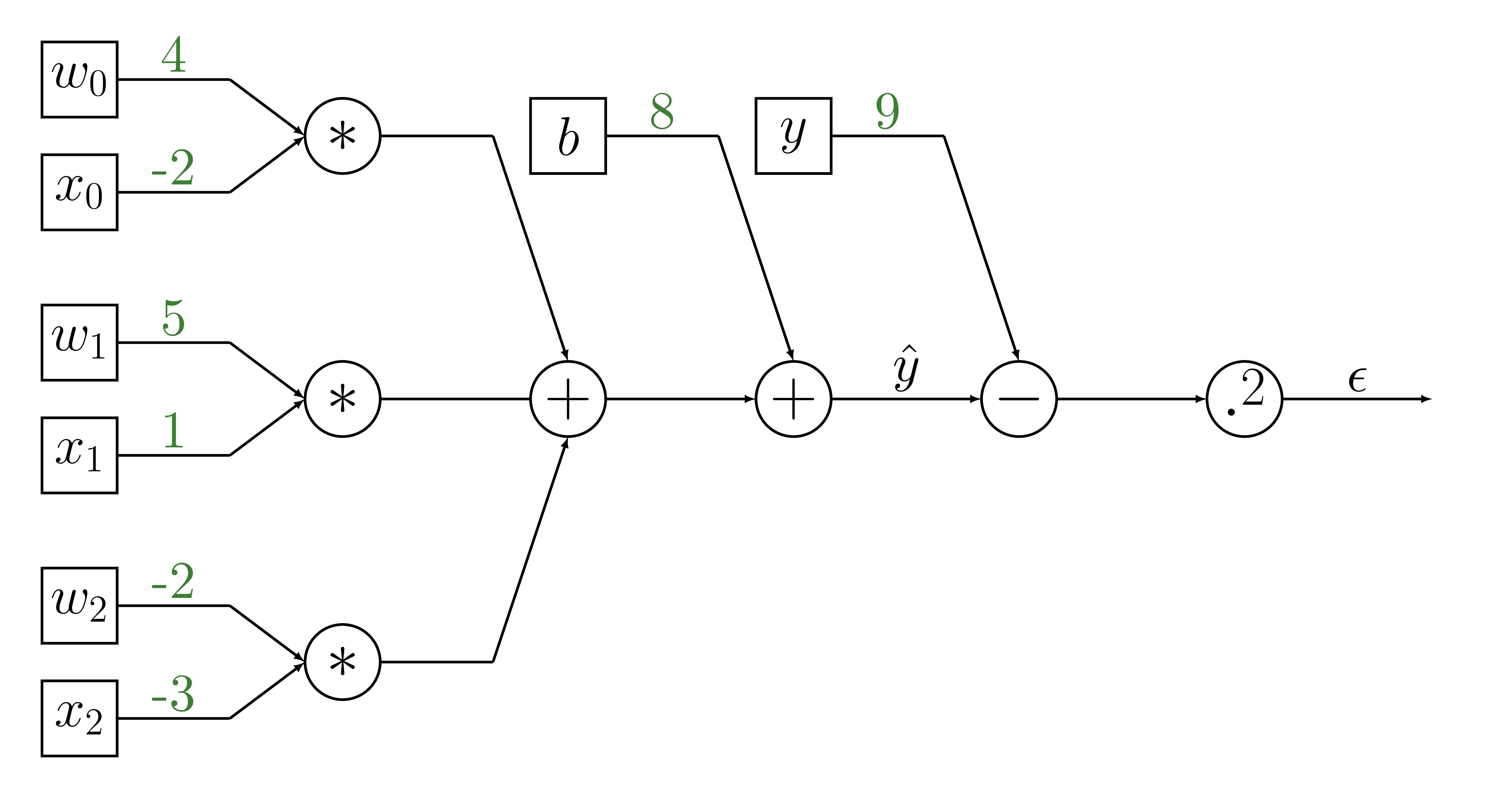
Forward propagation
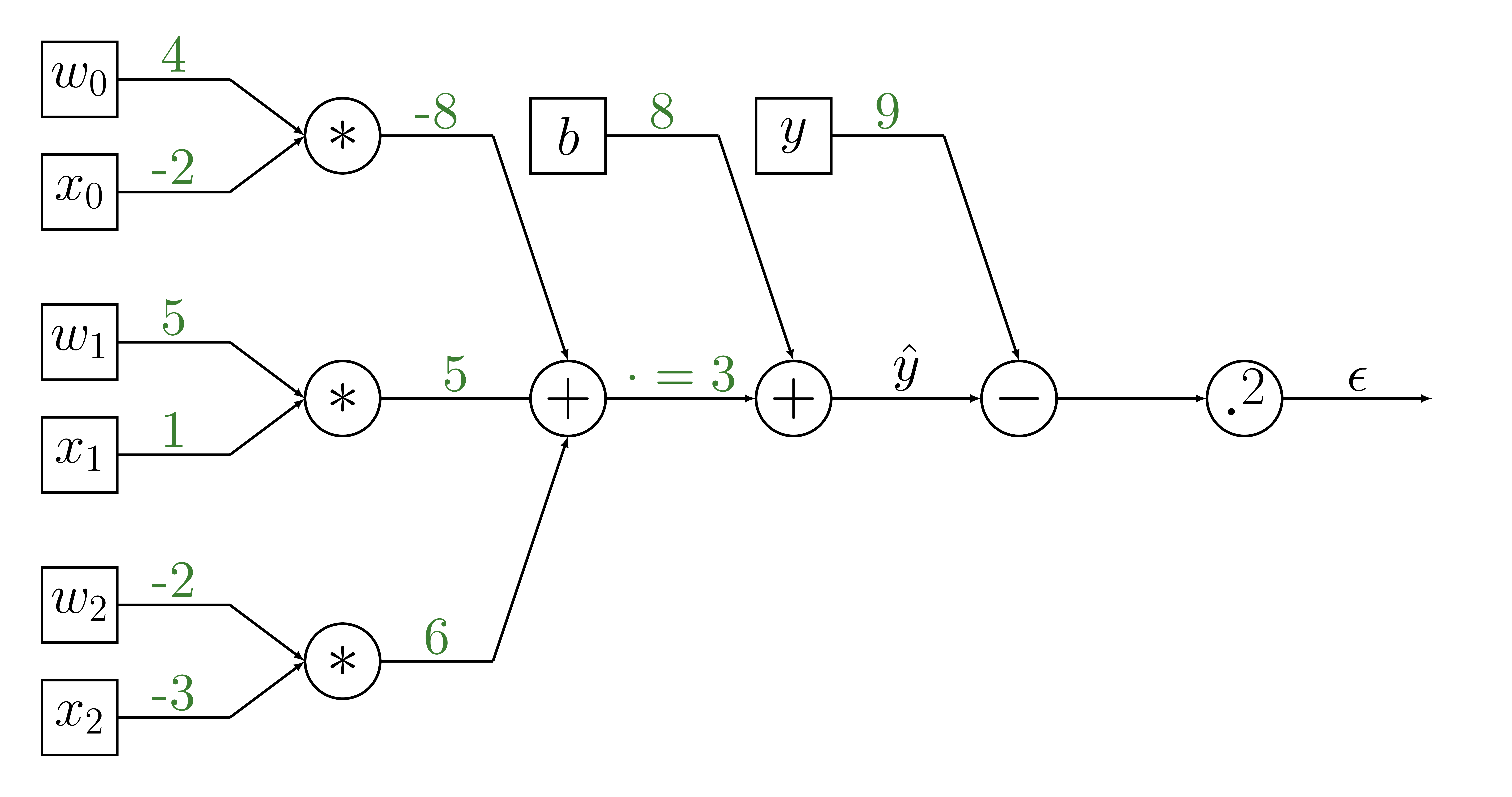
Forward propagation

Forward propagation
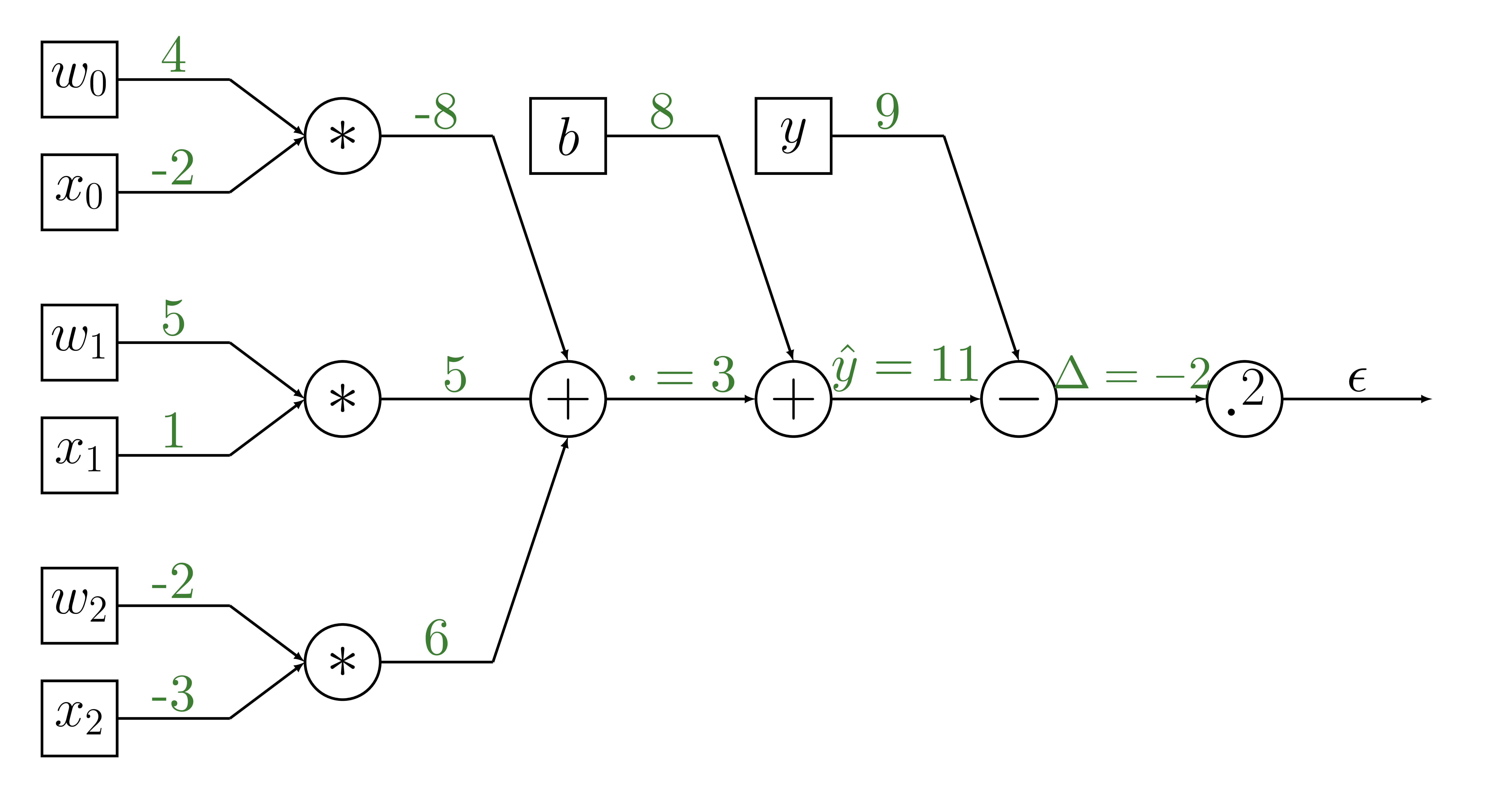
Forward propagation
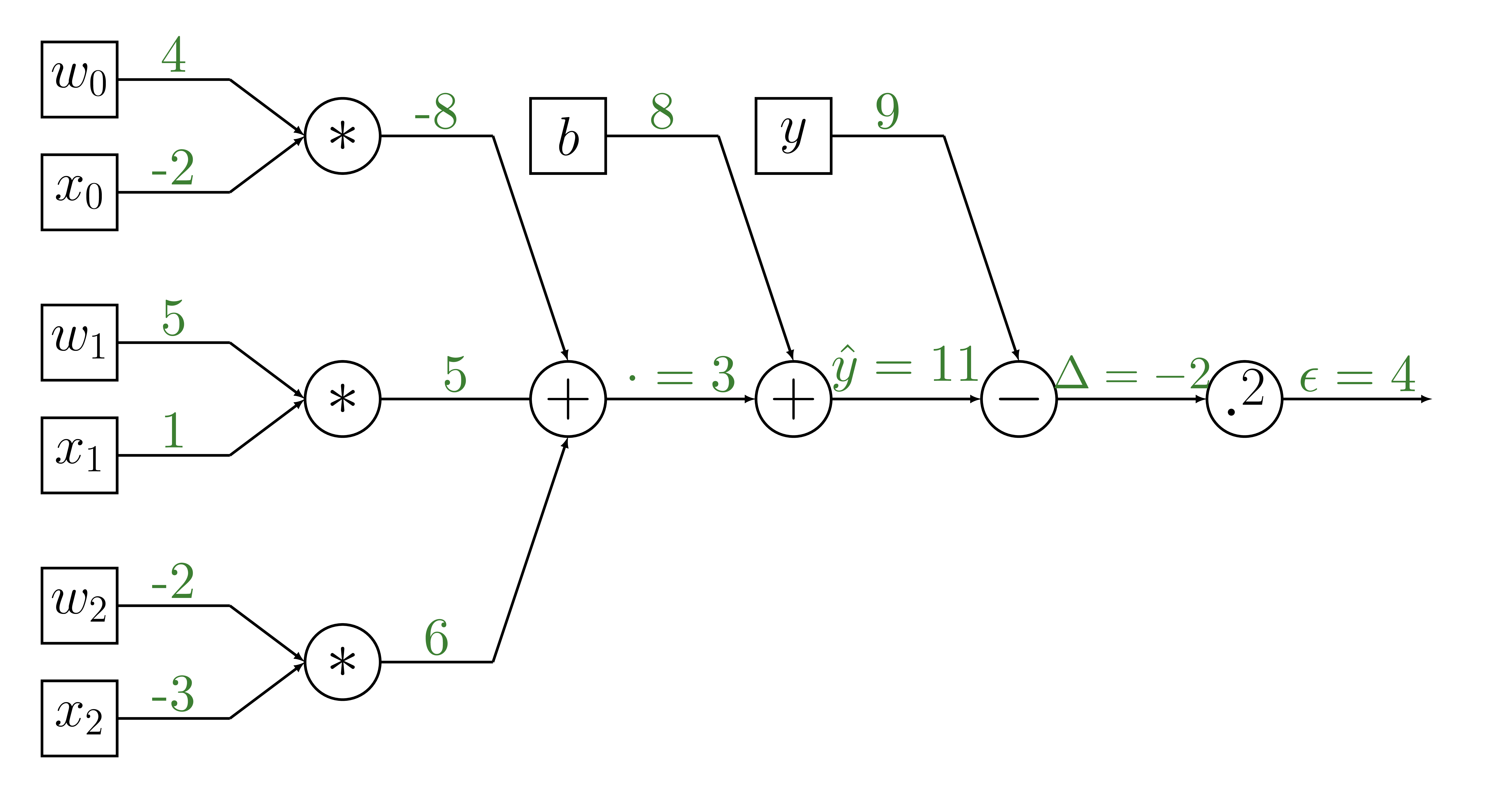
Forward propagation
	def training_round(x, y, weights, intercept,
	                   alpha=learning_rate):
      # calculate our estimate
      y_hat = model(x, weights, intercept)

      # calculate error
      delta_y = y - y_hat

      # calculate gradients
      gradient_weights = -2 * delta_y * weights
      gradient_intercept = -2 * delta_y

      # update parameters
      weights = weights - alpha * gradient_weights
      intercept = intercept - alpha * gradient_intercept

      return weights, intercept
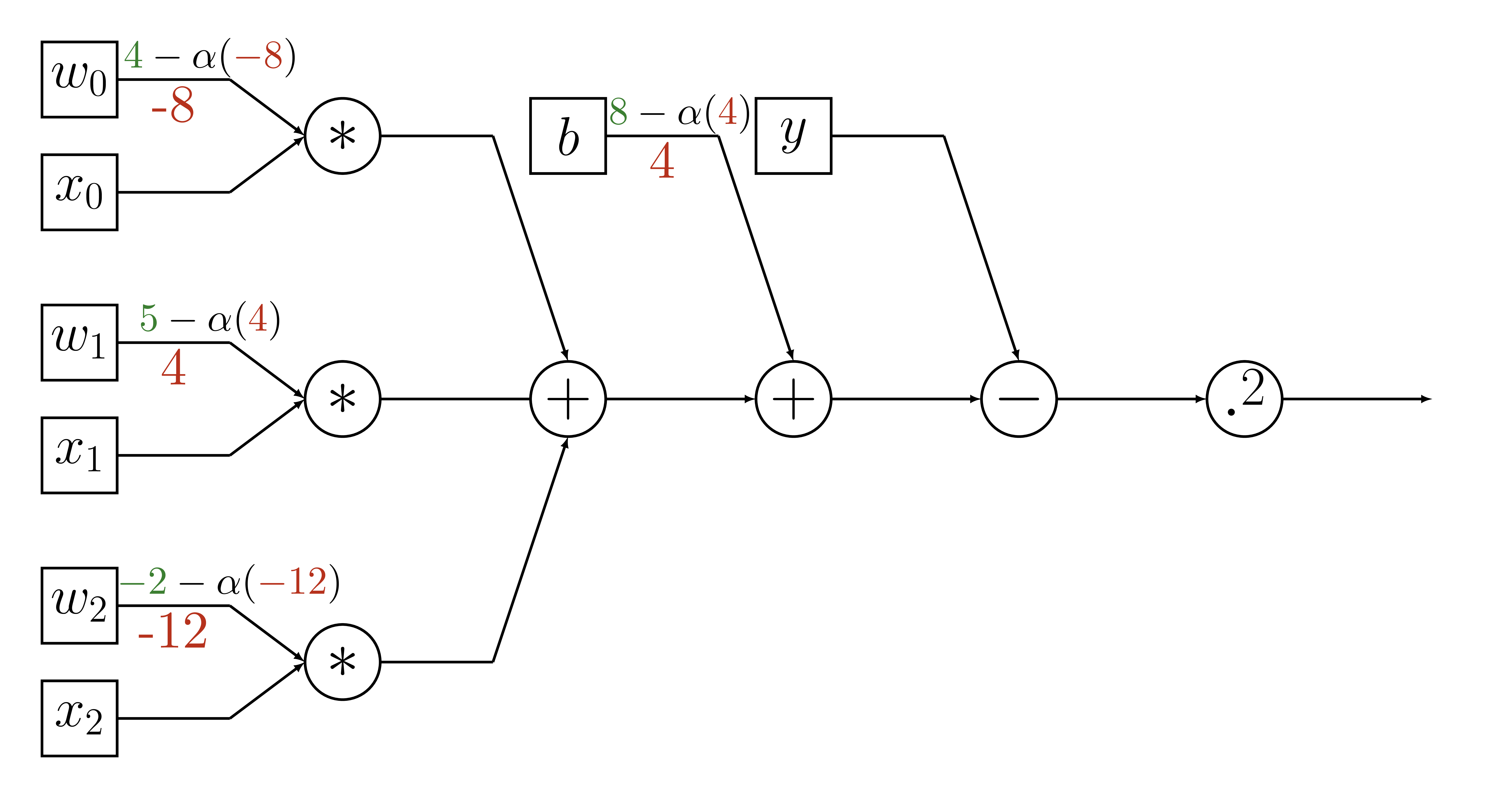
Backpropagation
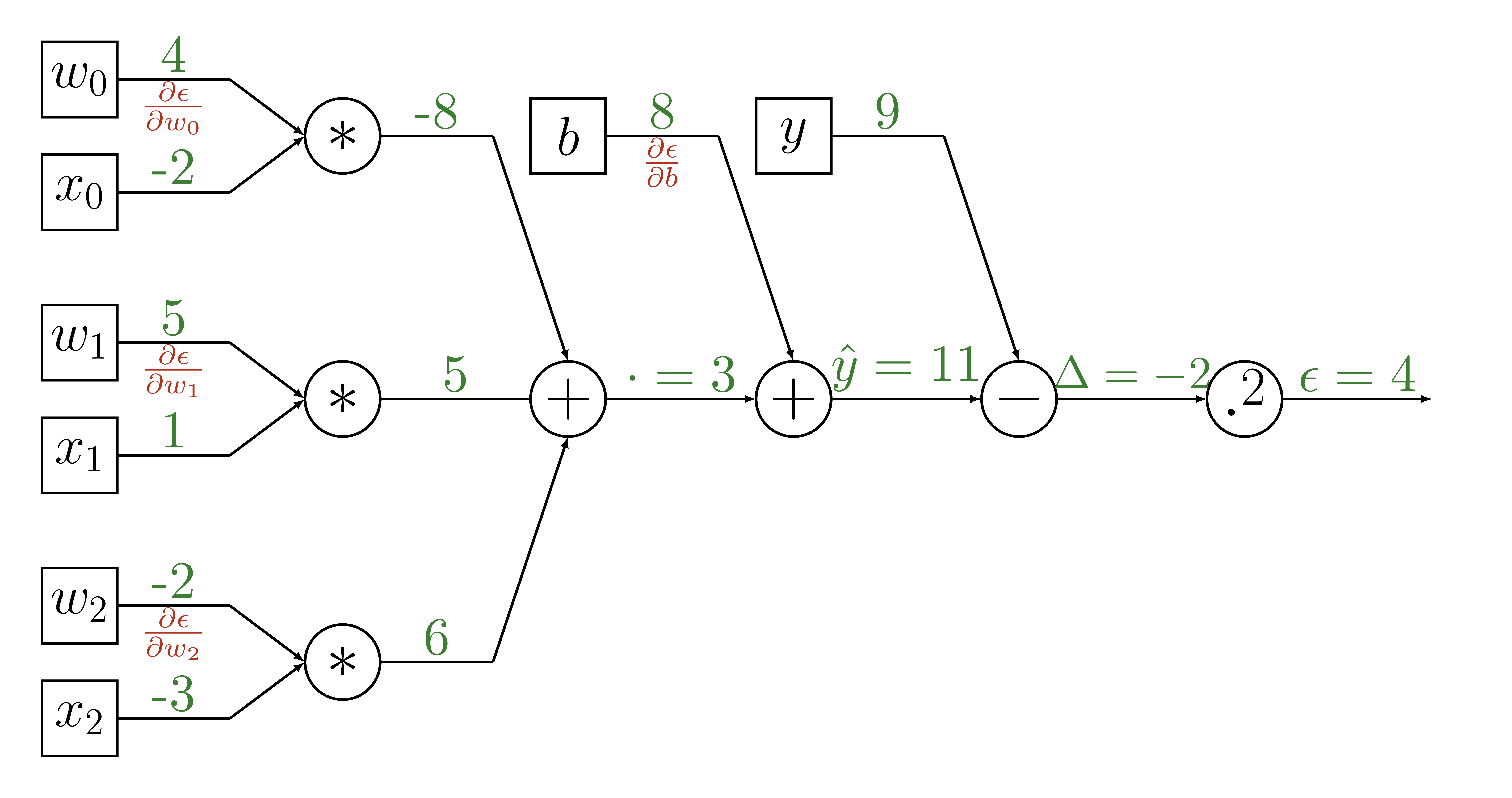
Backpropagation
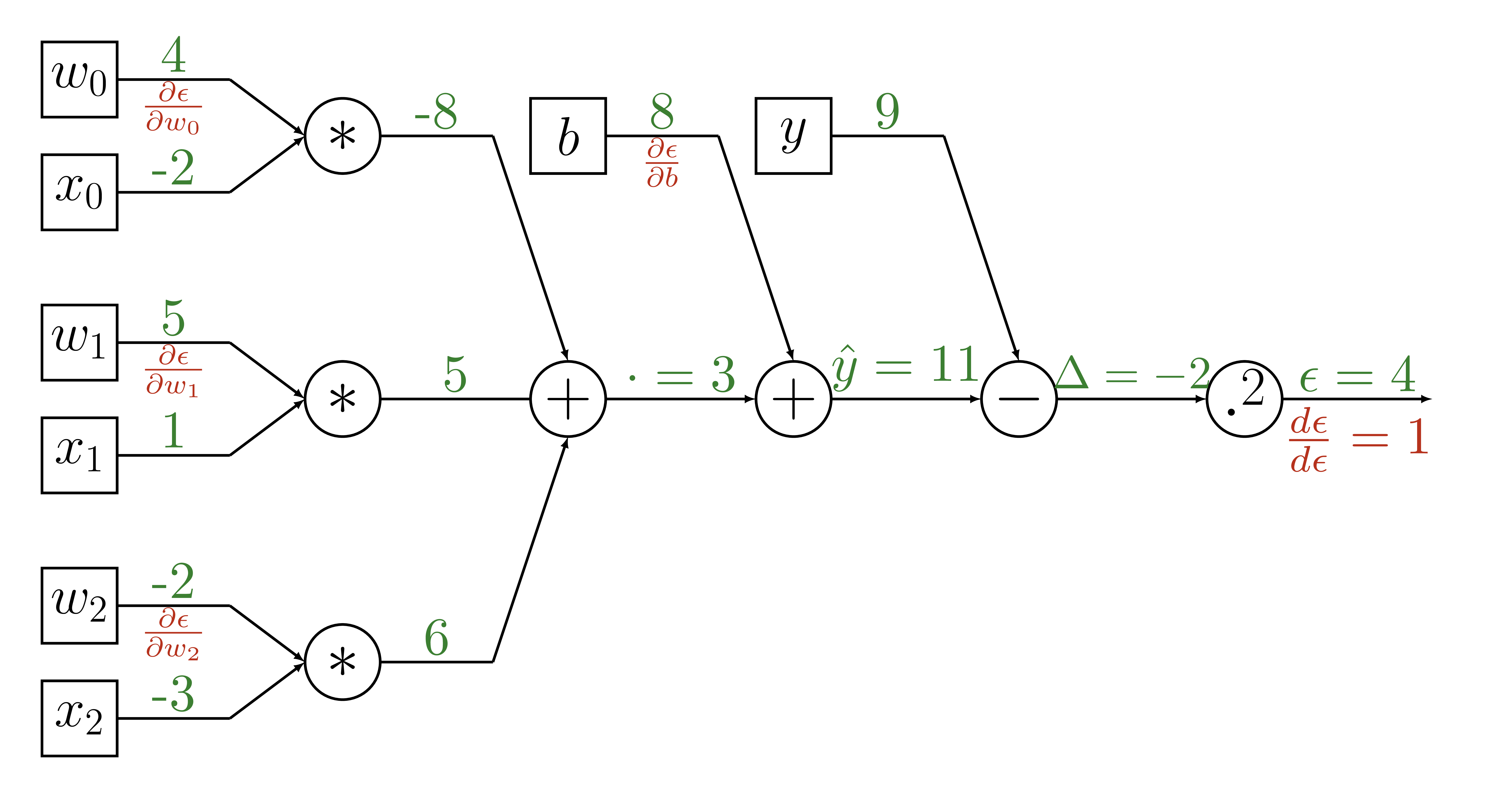
Backpropagation
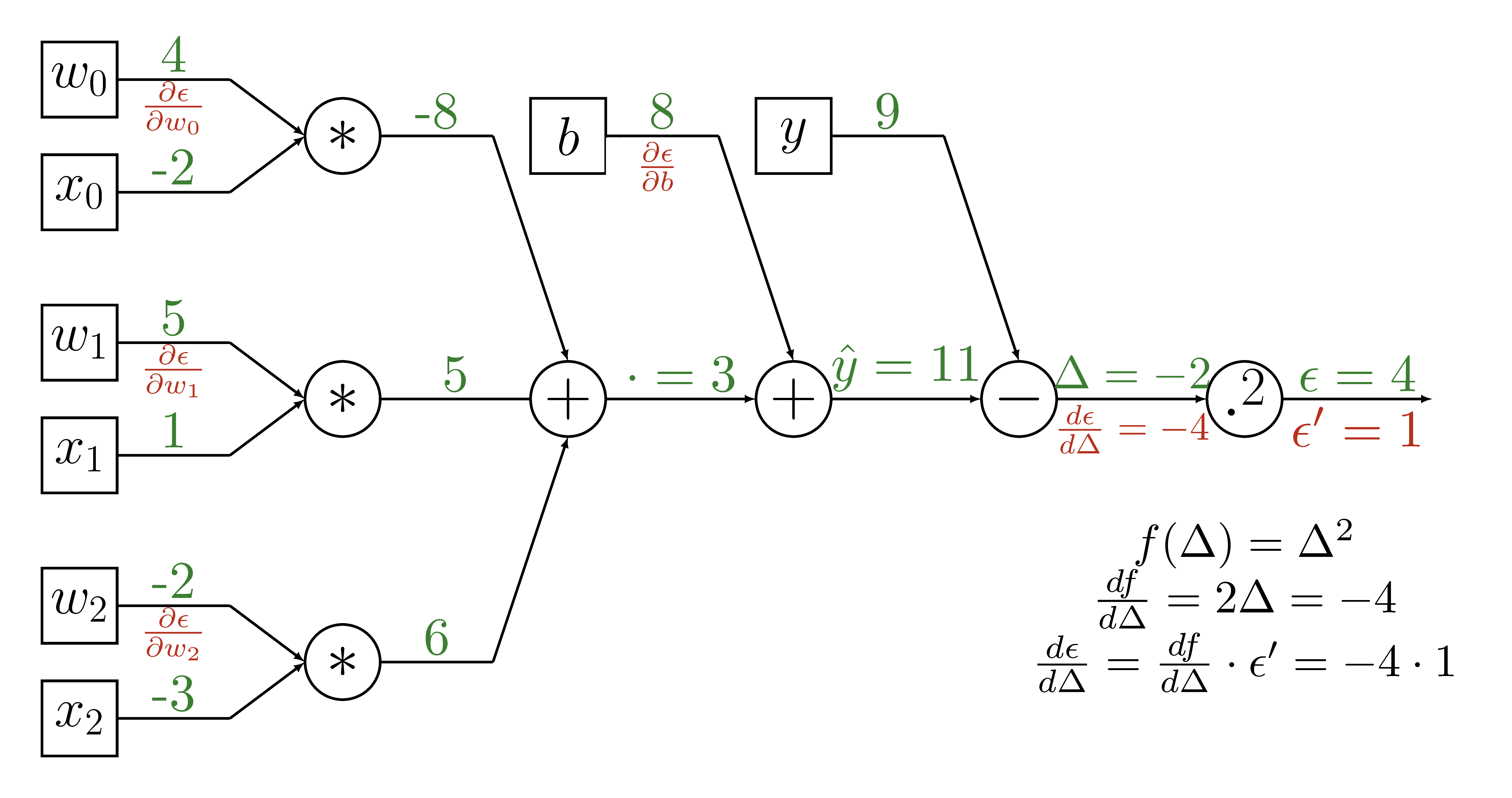
Backpropagation
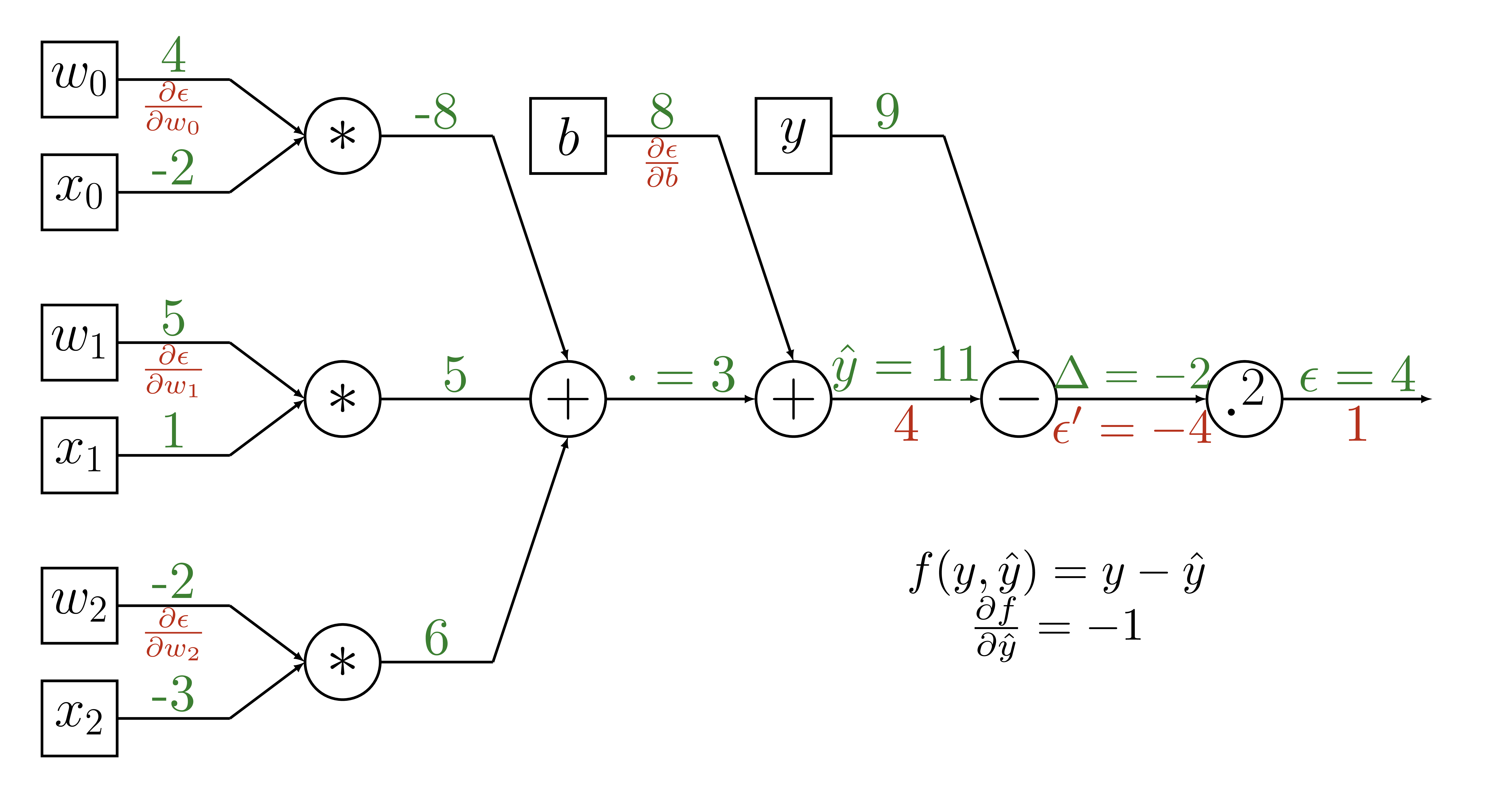
Backpropagation
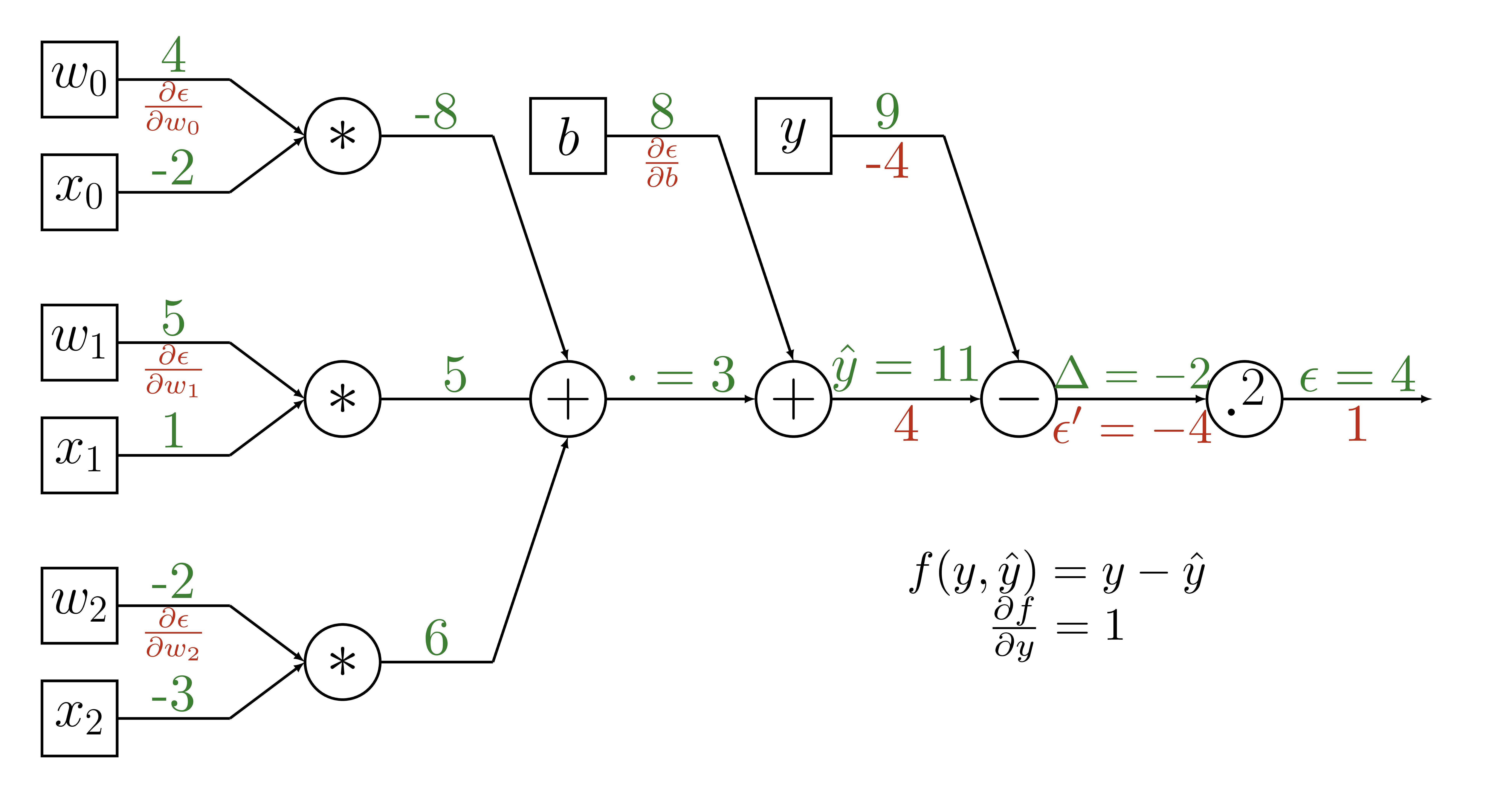
Backpropagation
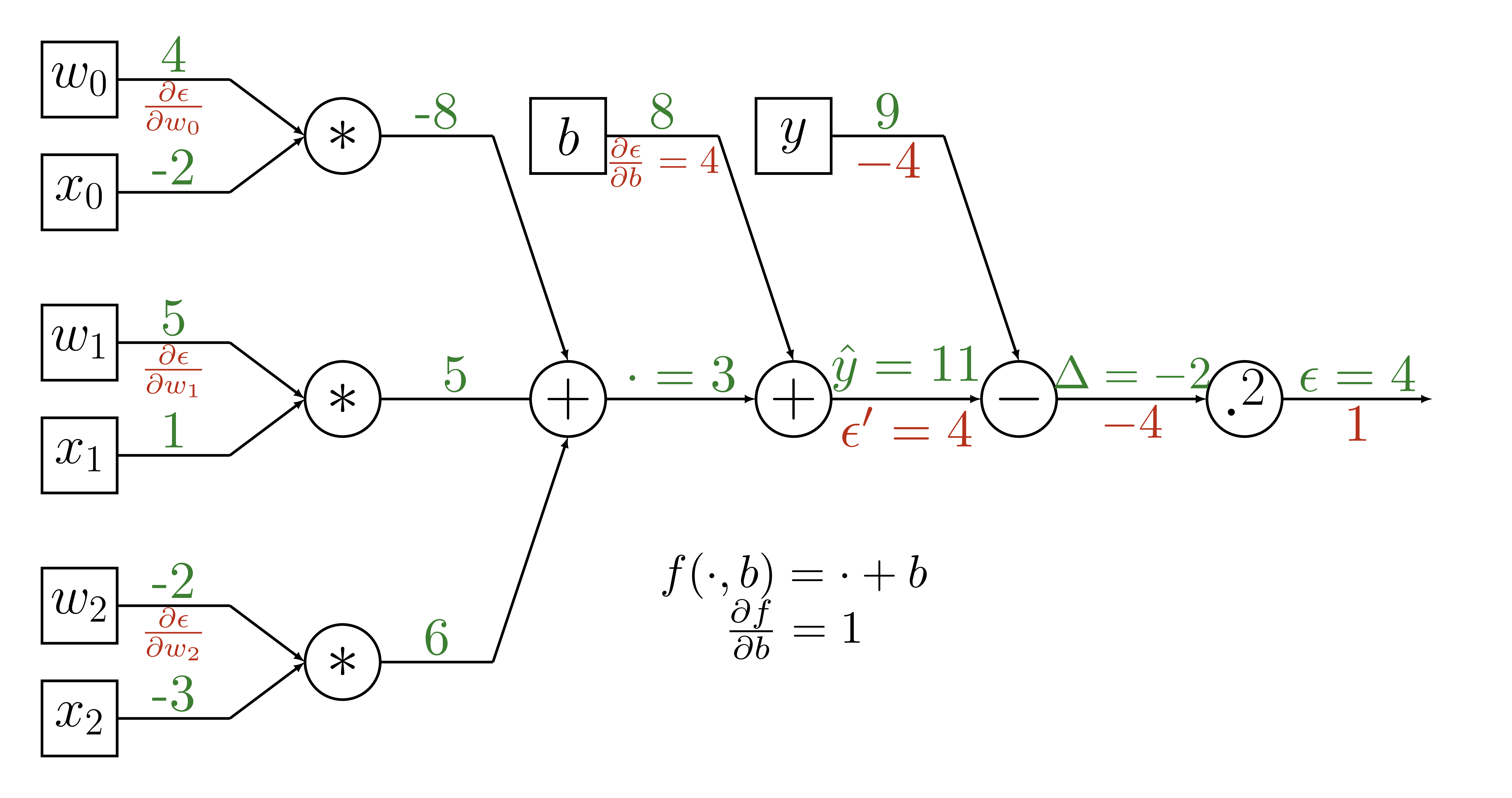
Backpropagation
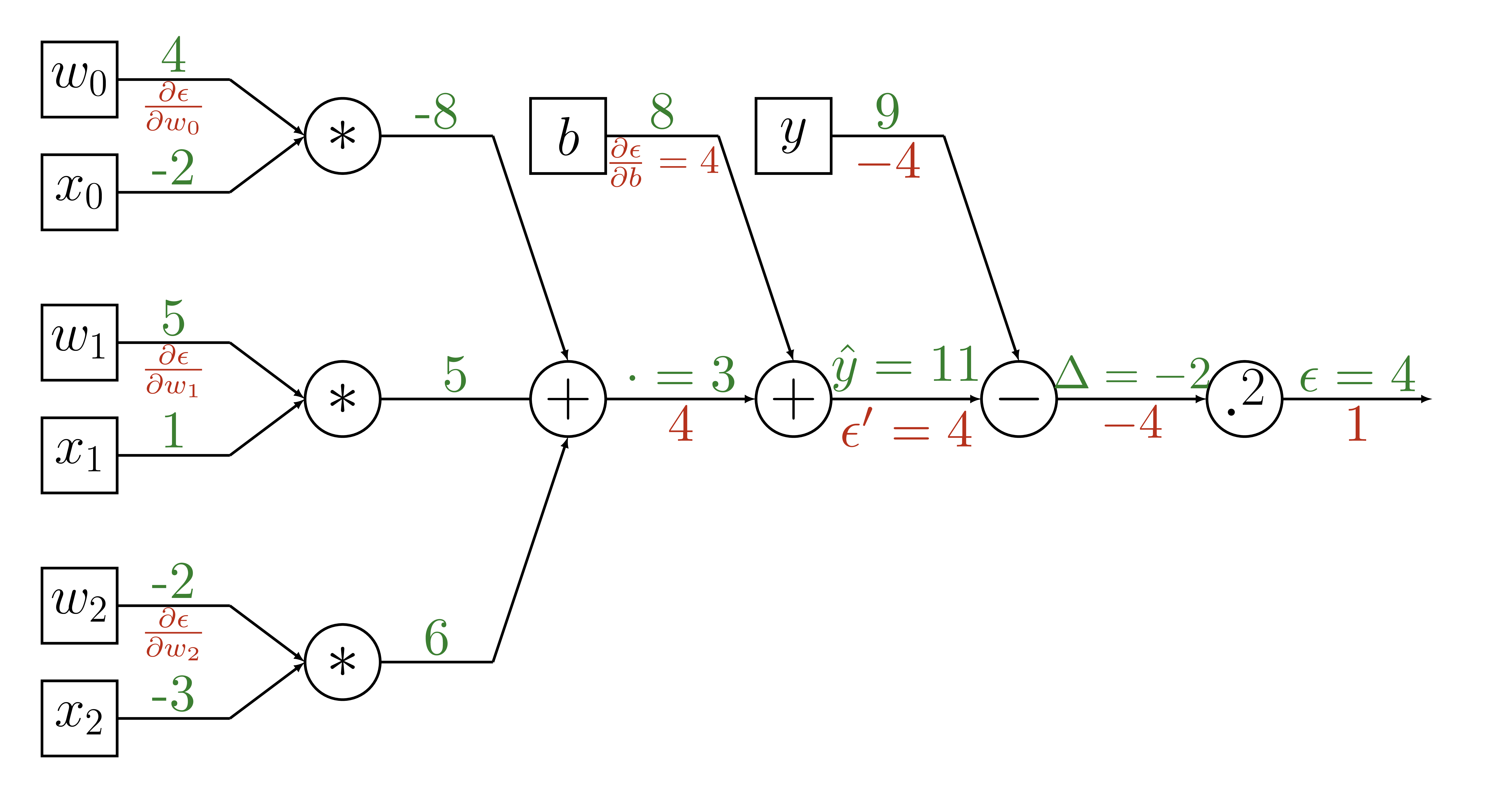
Backpropagation
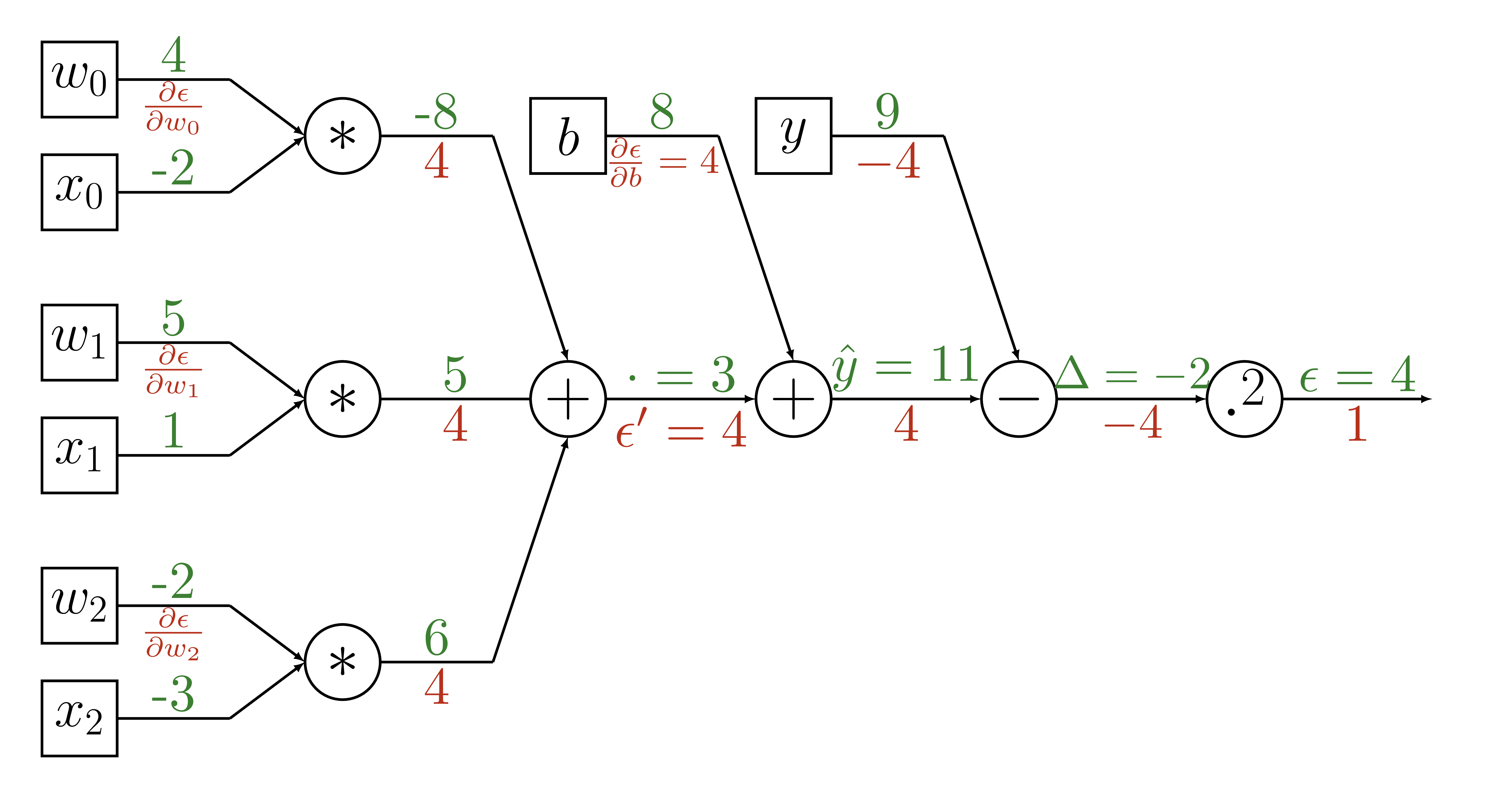
Backpropagation
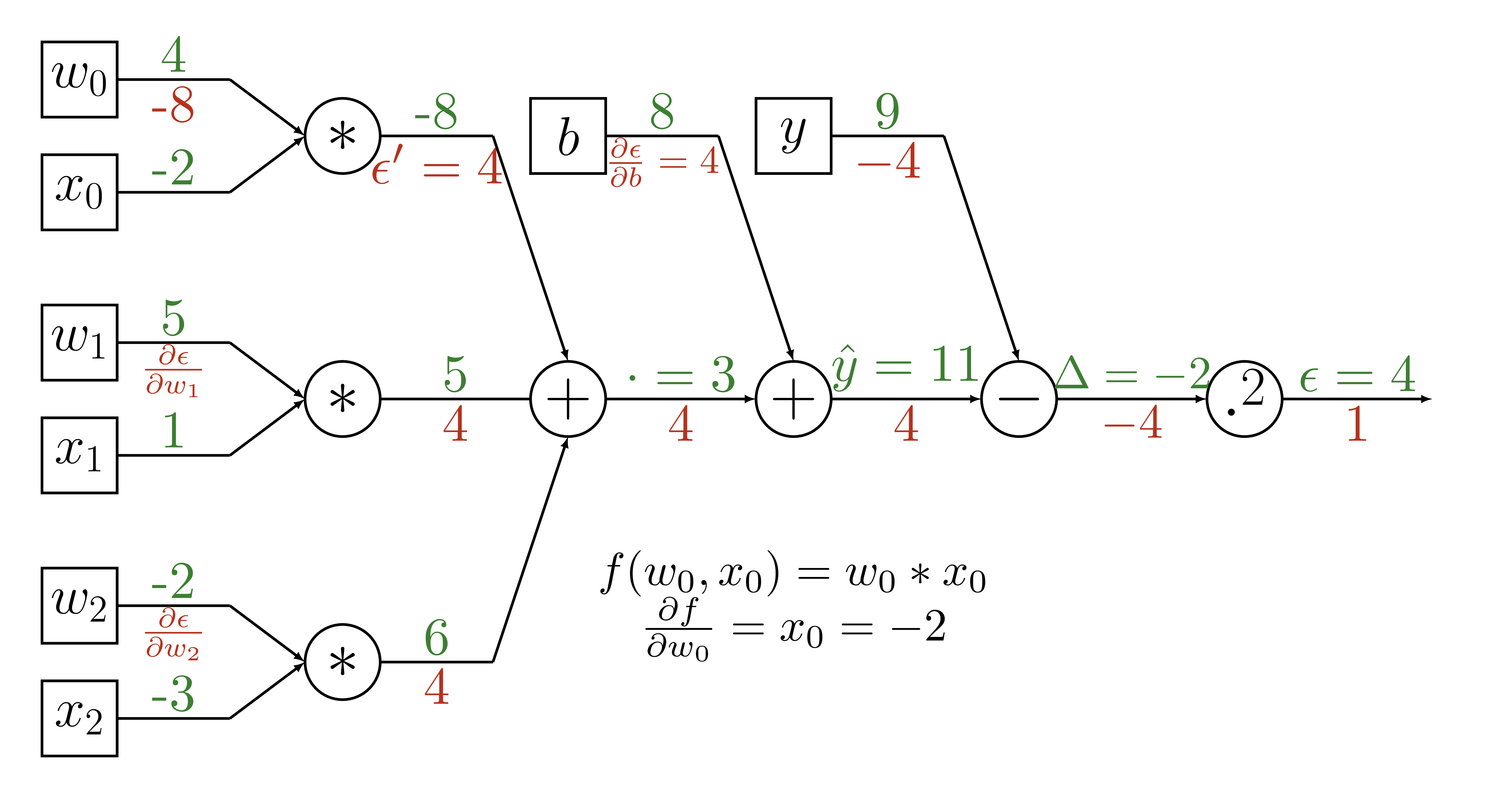
Backpropagation
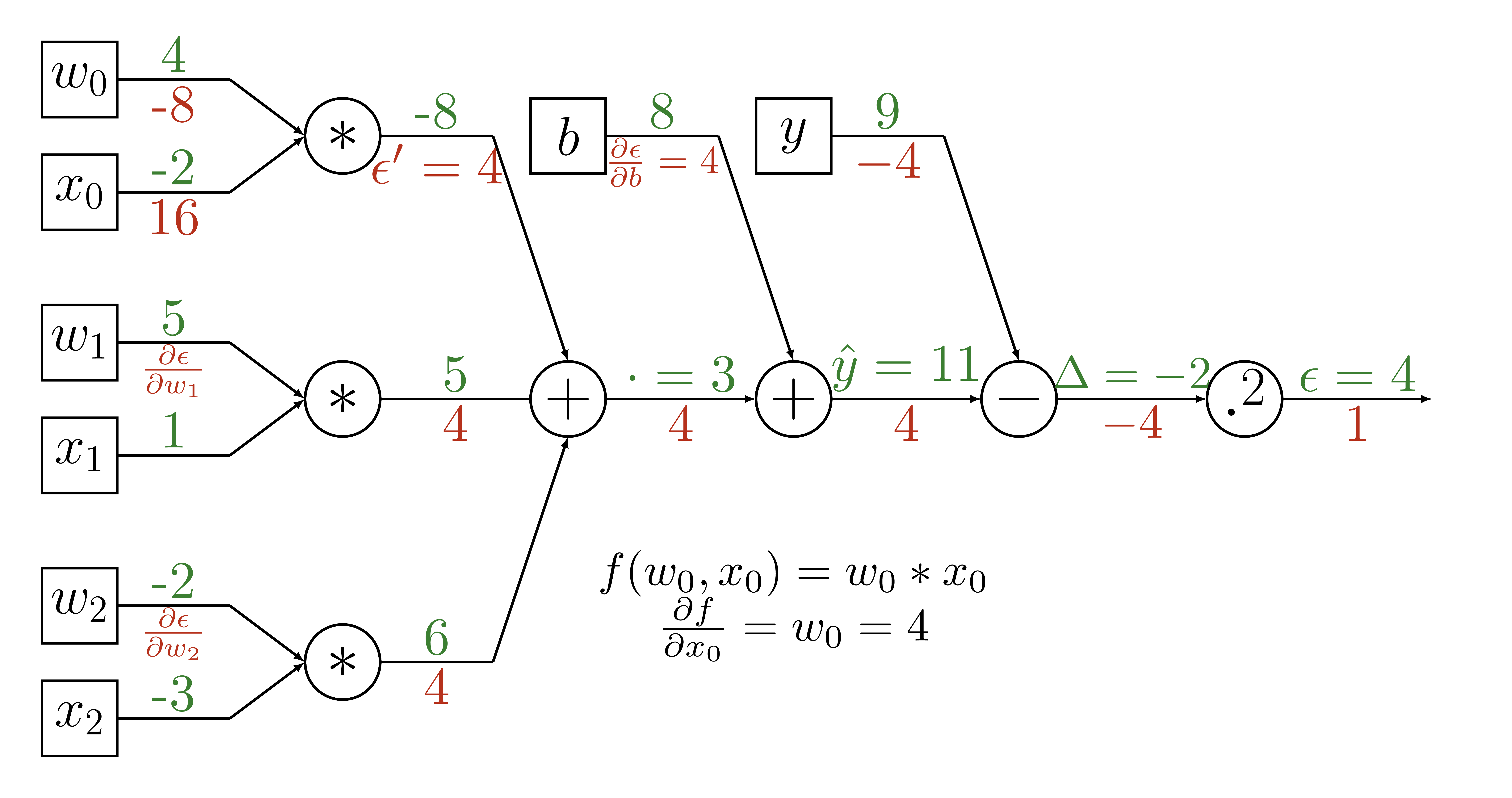
Backpropagation
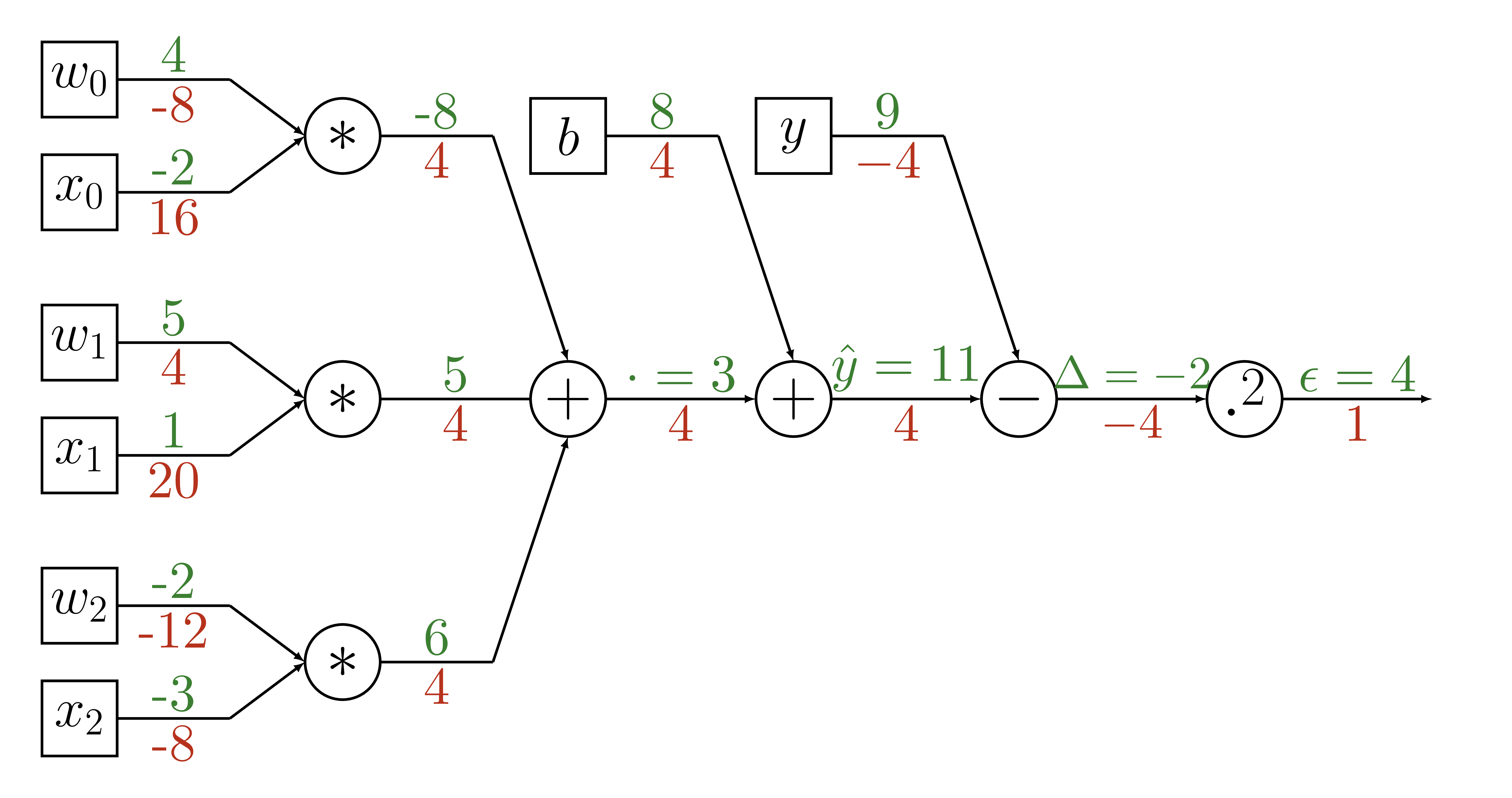
Backpropagation
	def training_round(x, y, weights, intercept,
	                   alpha=learning_rate):
      # calculate our estimate
      y_hat = model(x, weights, intercept)

      # calculate error
      delta_y = y - y_hat

      # calculate gradients
      gradient_weights = -2 * delta_y * weights
      gradient_intercept = -2 * delta_y

      # update parameters
      weights = weights - alpha * gradient_weights
      intercept = intercept - alpha * gradient_intercept

      return weights, intercept
Variable Update
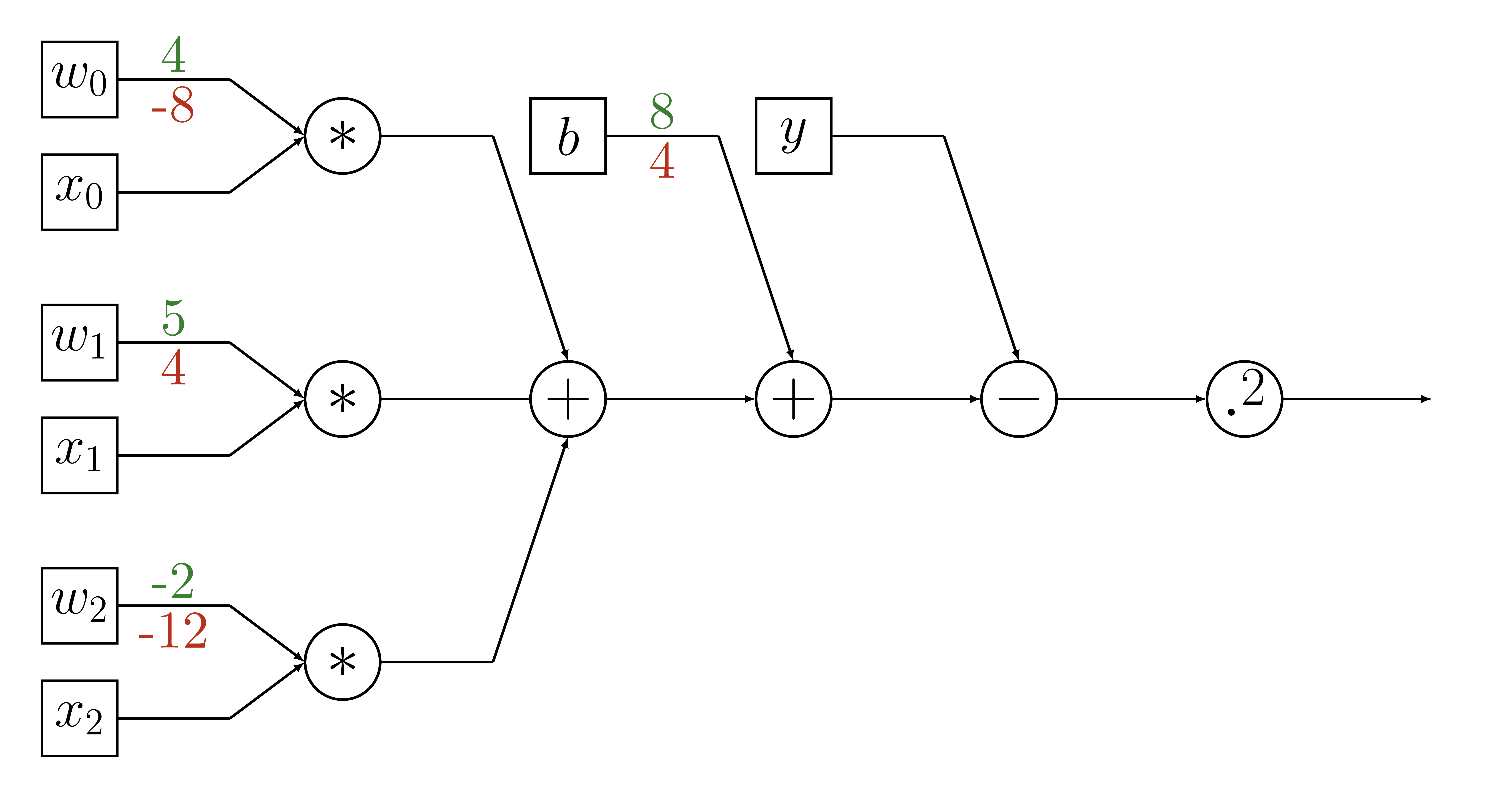
Variable Update
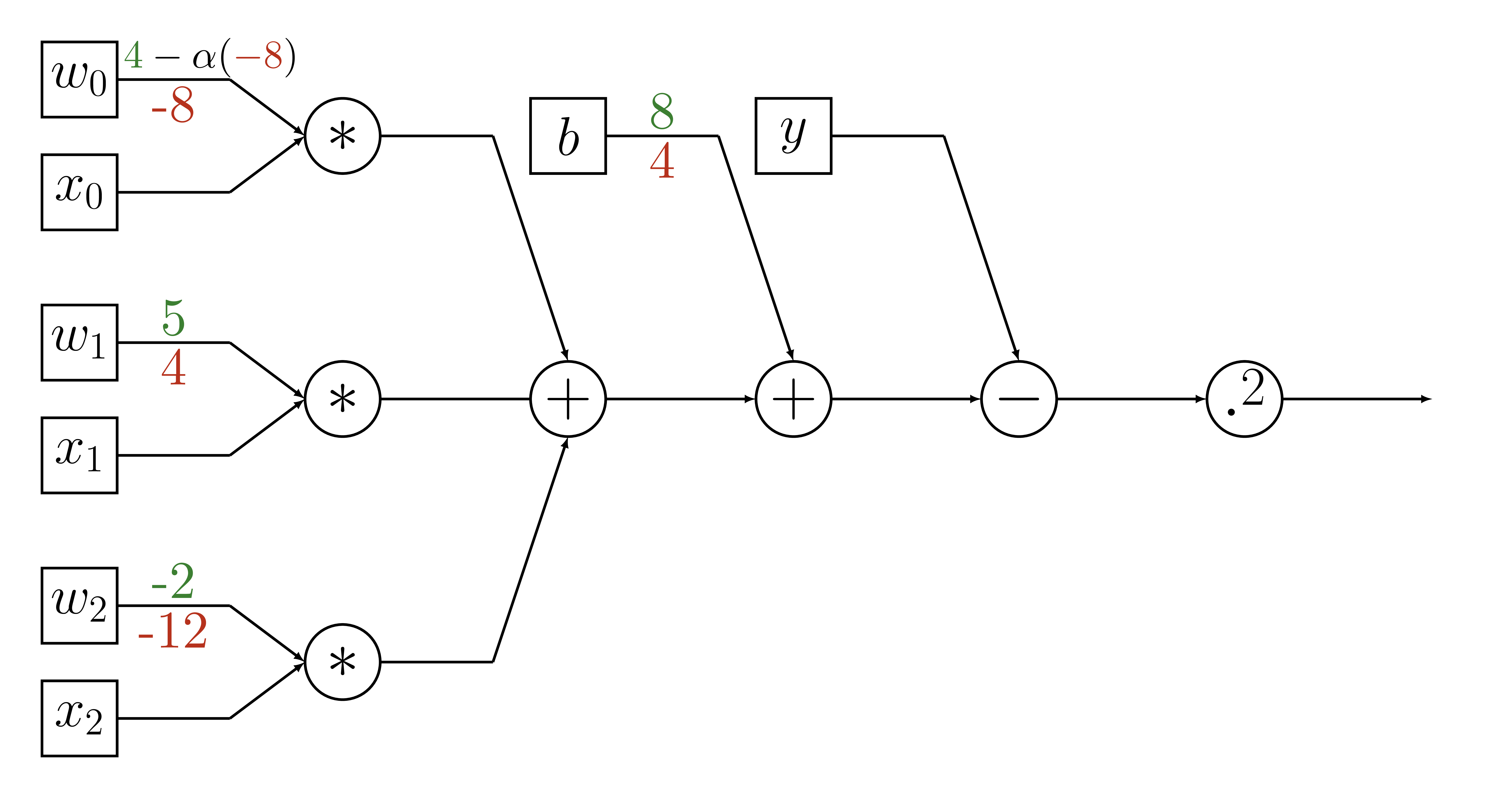
Variable Update
Variable Update
def training_round(x, y, weights, intercept,
                   alpha=learning_rate):
    # calculate our estimate
    y_hat = model(x, weights, intercept)

    # calculate error
    delta_y = y - y_hat

    # calculate gradients
    gradient_weights = -2 * delta_y * weights
    gradient_intercept = -2 * delta_y

    # update parameters
    weights = weights - alpha * gradient_weights
    intercept = intercept - alpha * gradient_intercept

    return weights, intercept
Numpy → TensorFlow
sess.run(optimizer,
         feed_dict={
             X: X_batch,
             Y: Y_batch
         })
Testing
with tf.Session() as sess:
    # train
    # ... (code from above)

    # test
    Y_predicted = sess.run(model,
                    feed_dict = {X: X_test})
    squared_error = tf.reduce_mean(
                 tf.square(Y_test, Y_predicted))

>>> np.sqrt(squared_error)
5967.39
Logistic regression
Problem
Binary classification
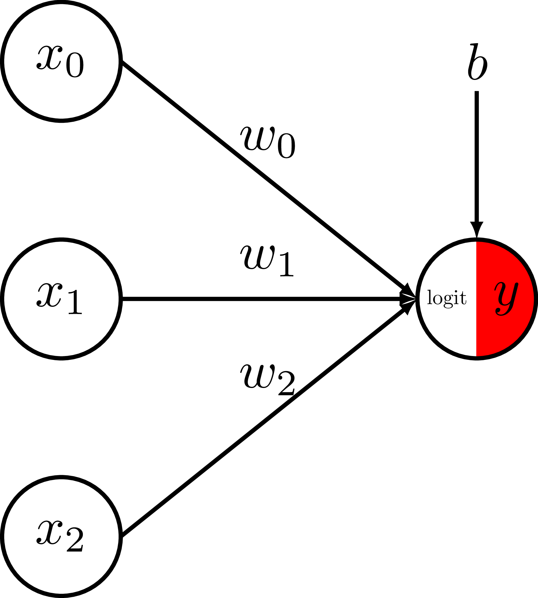
Binary logistic regression - Model
Take a weighted sum of the features
and add a bias term to get the logit.
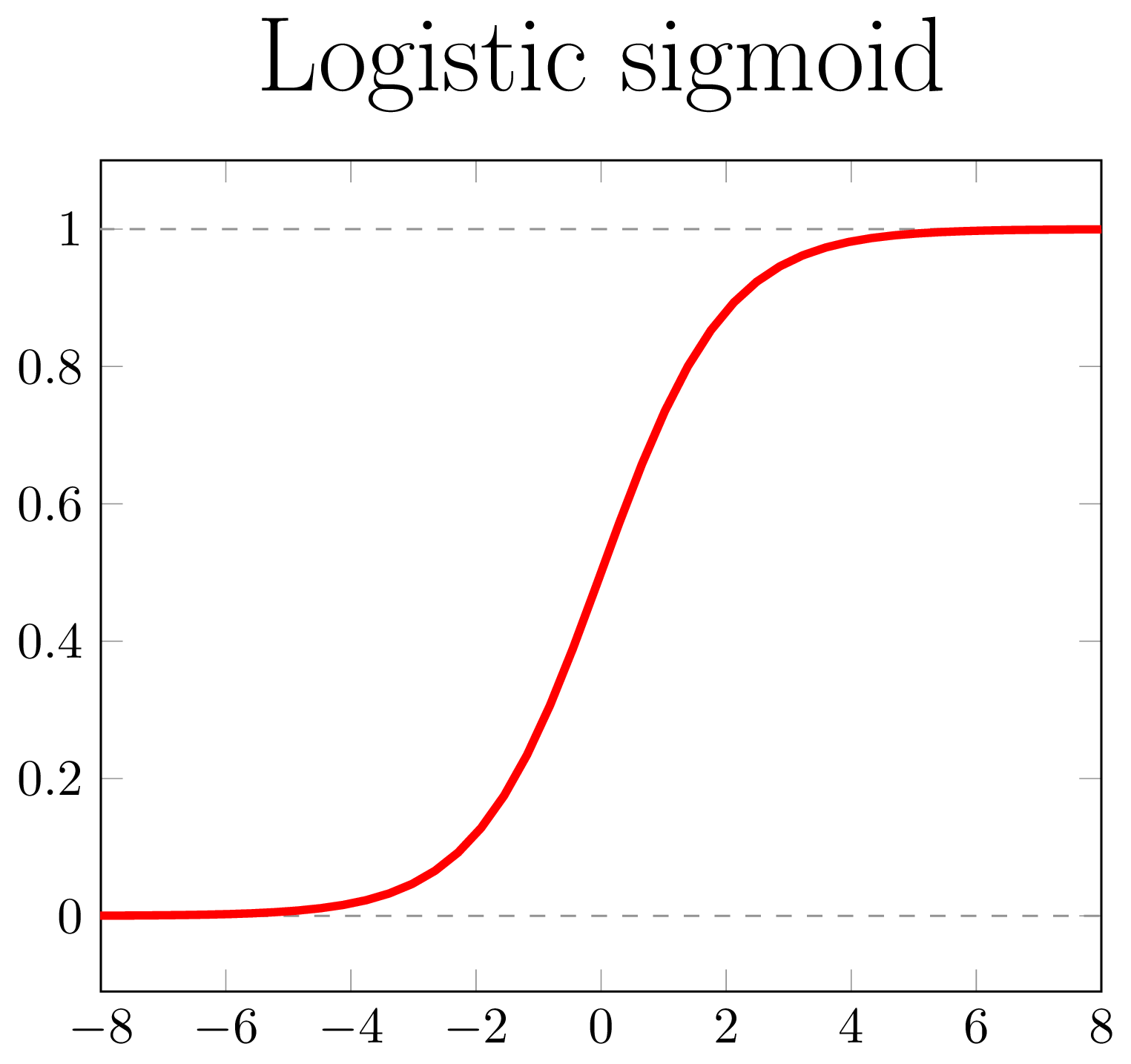
Convert the logit to a probability
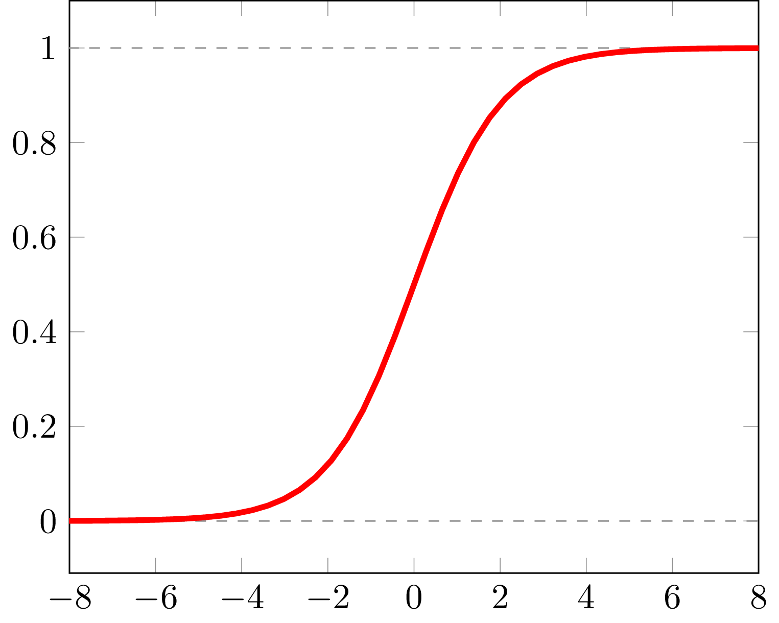
via the logistic-sigmoid function.
Binary logistic regression - Model
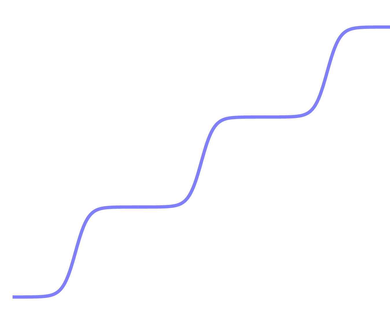
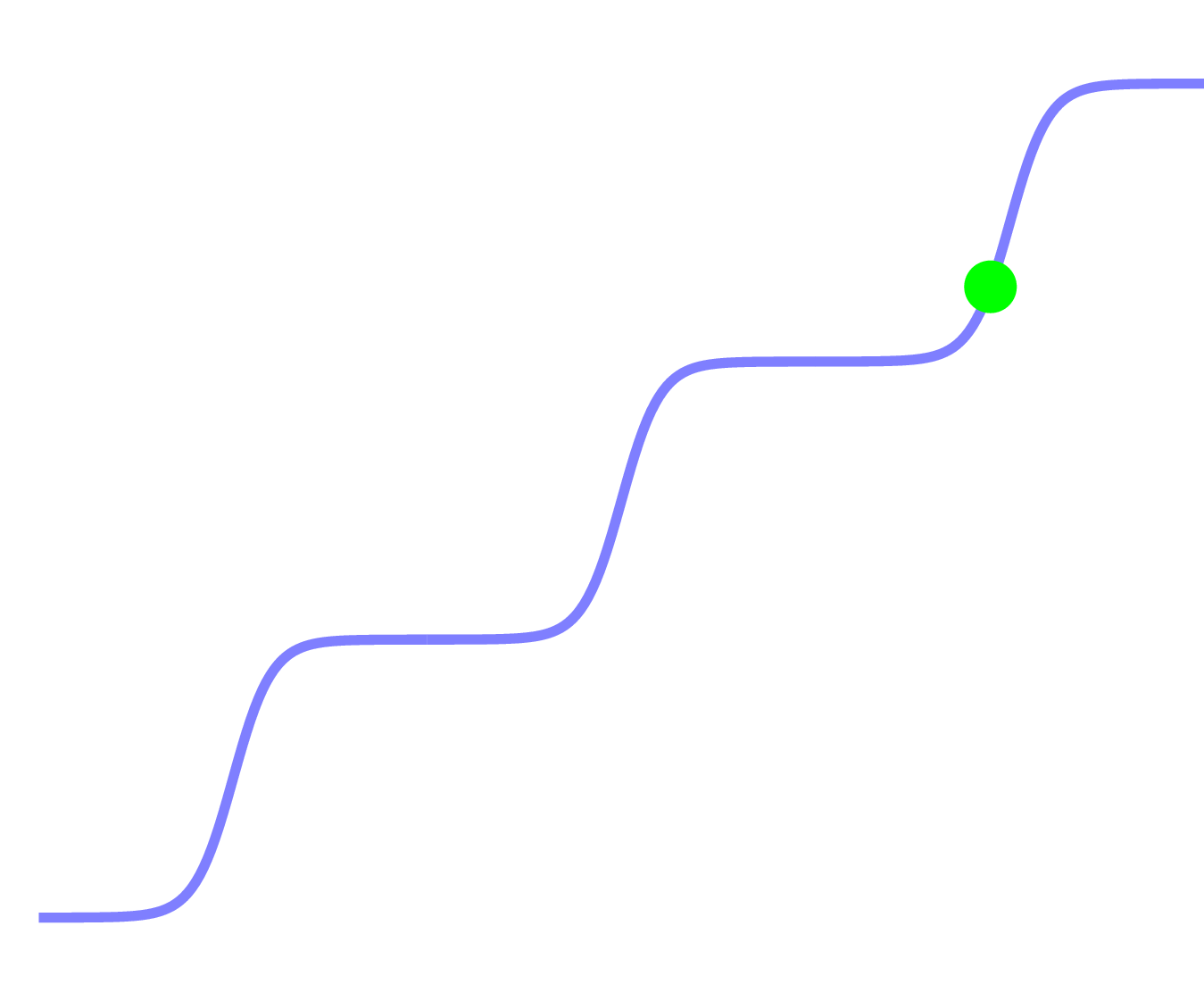
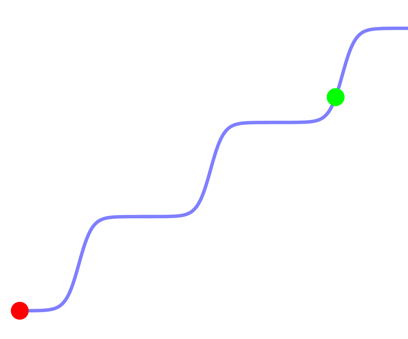
Logistic-sigmoid function
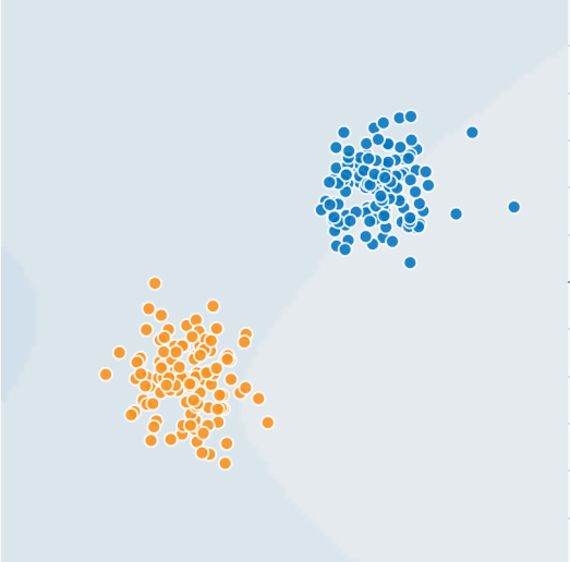
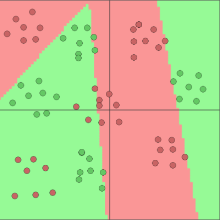
Classification with logistic regression
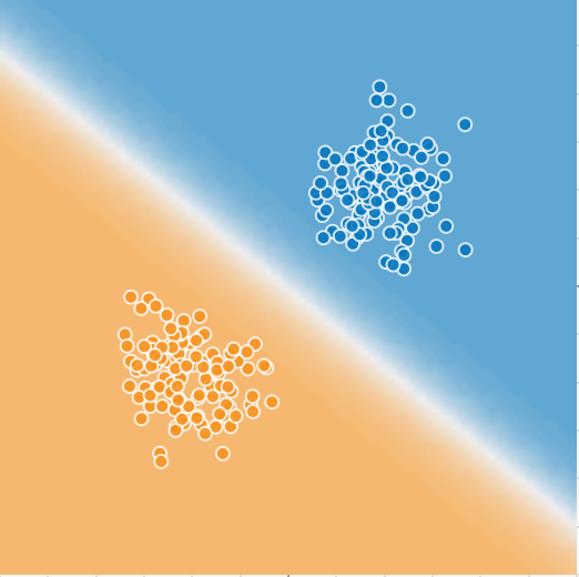
Image generated with playground.tensorflow.org
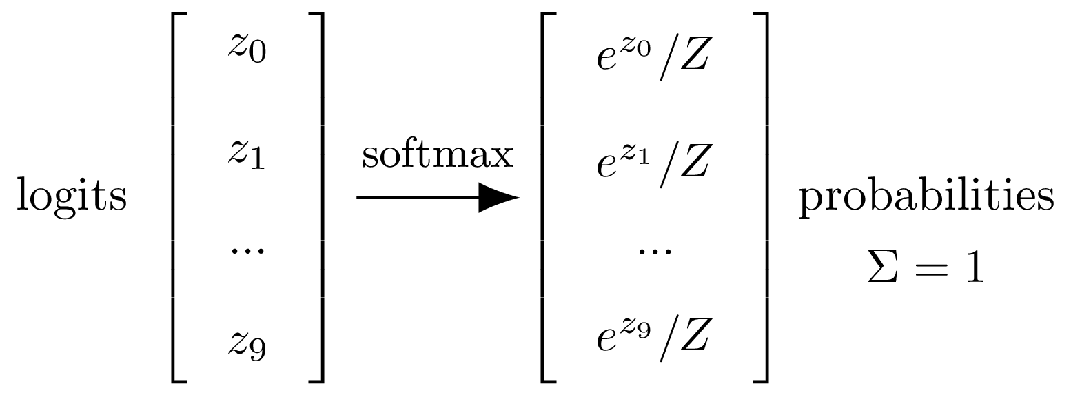
Model
Softmax
Z = np.sum(np.exp(logits))
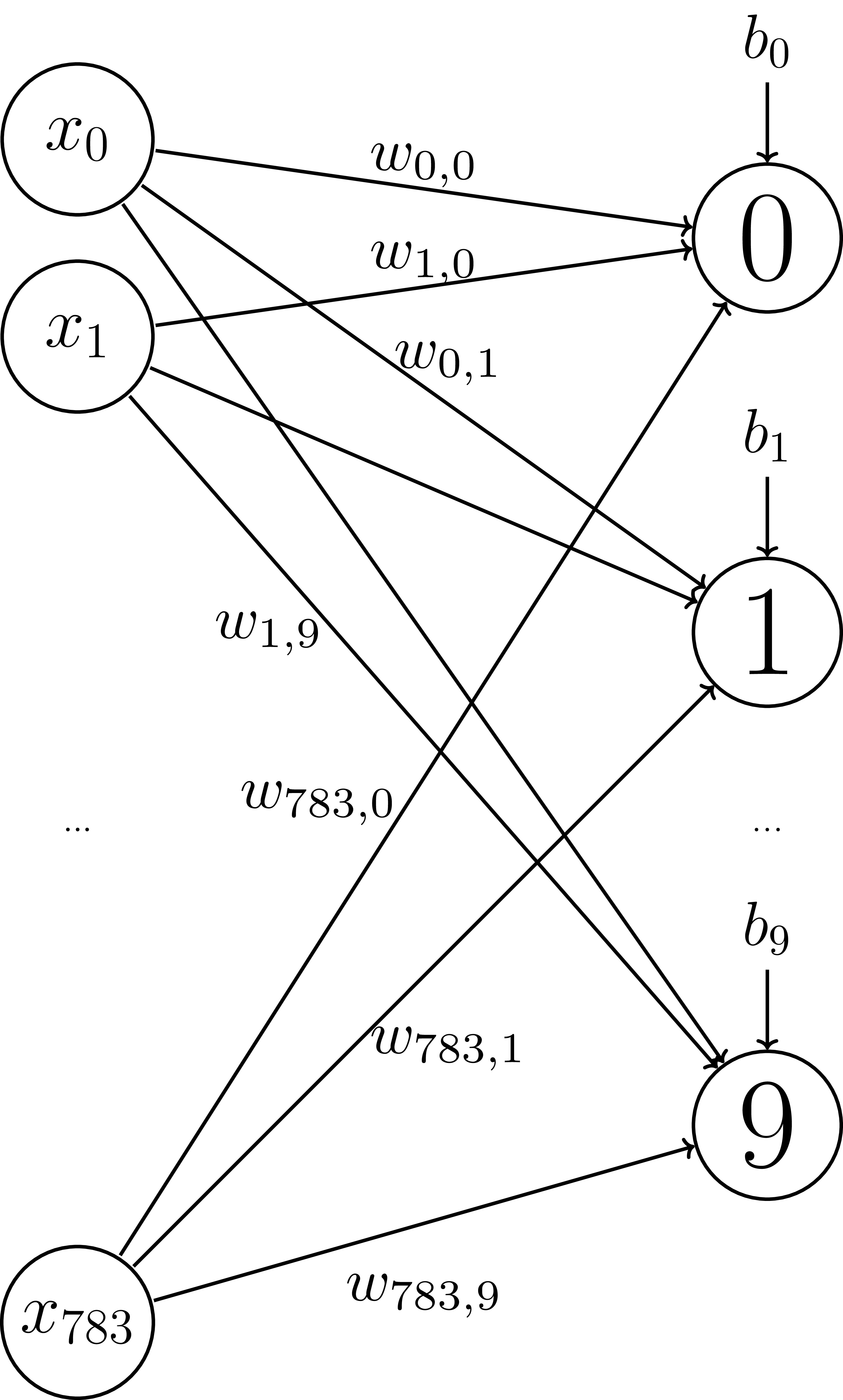
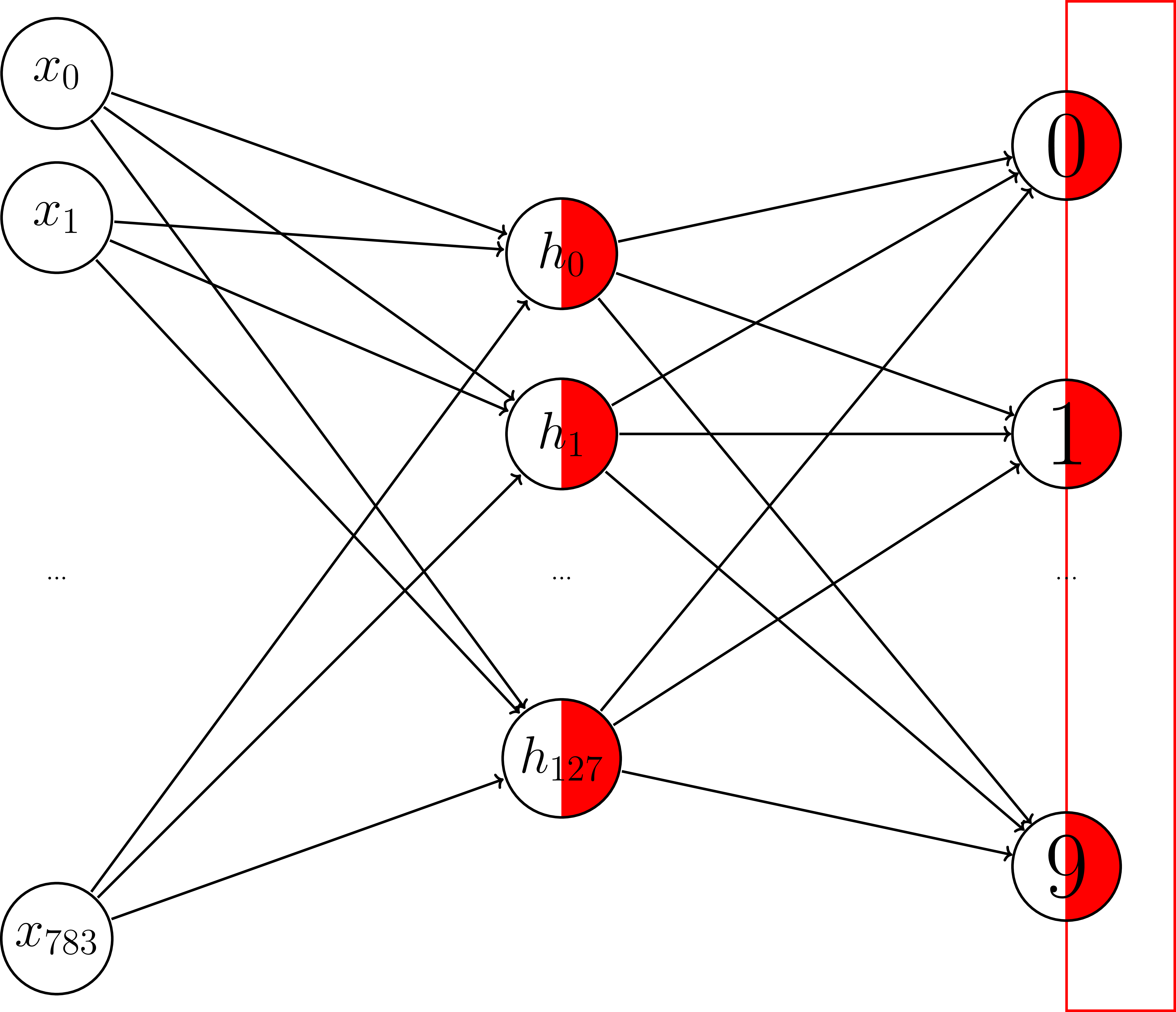
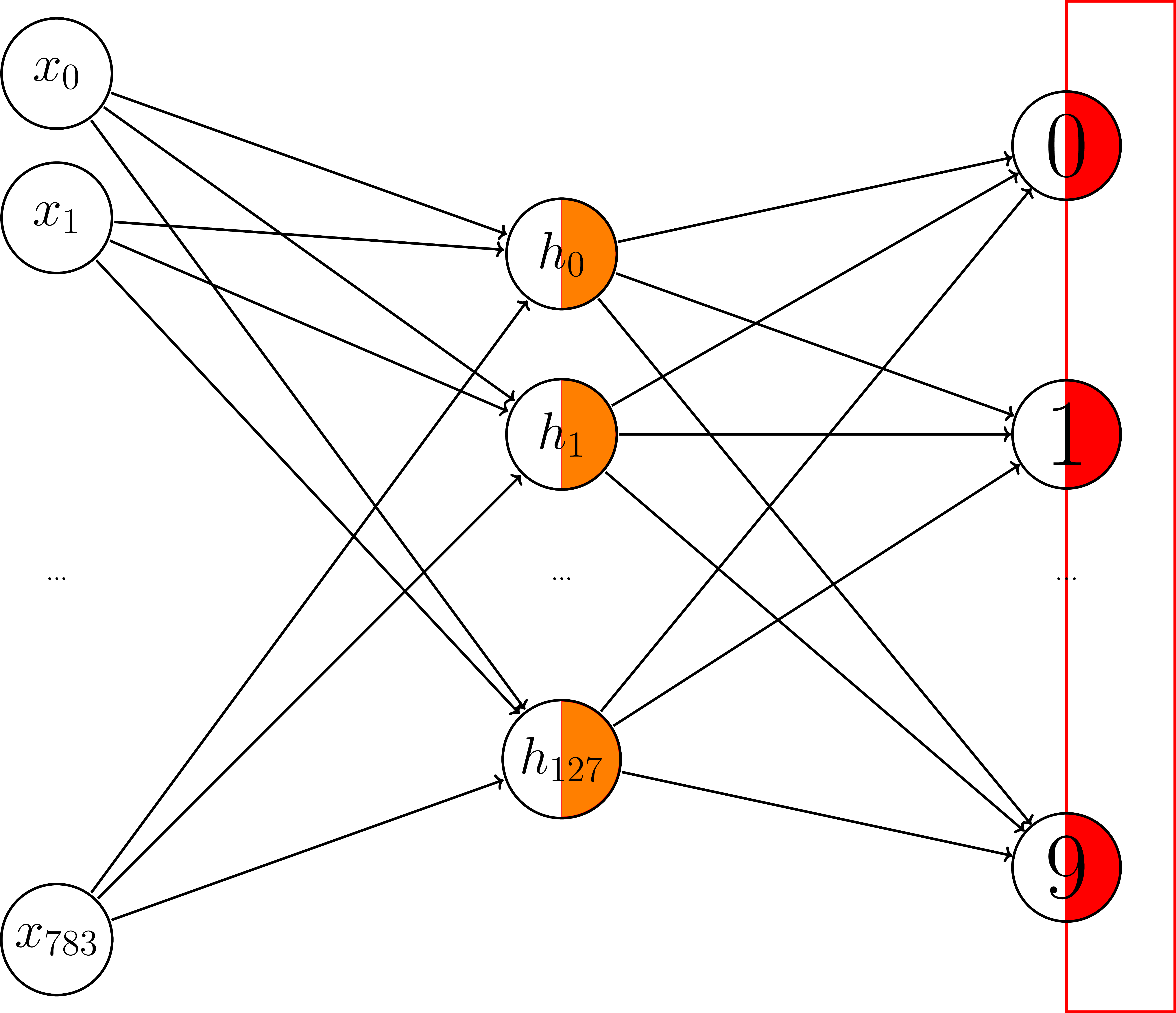
Model
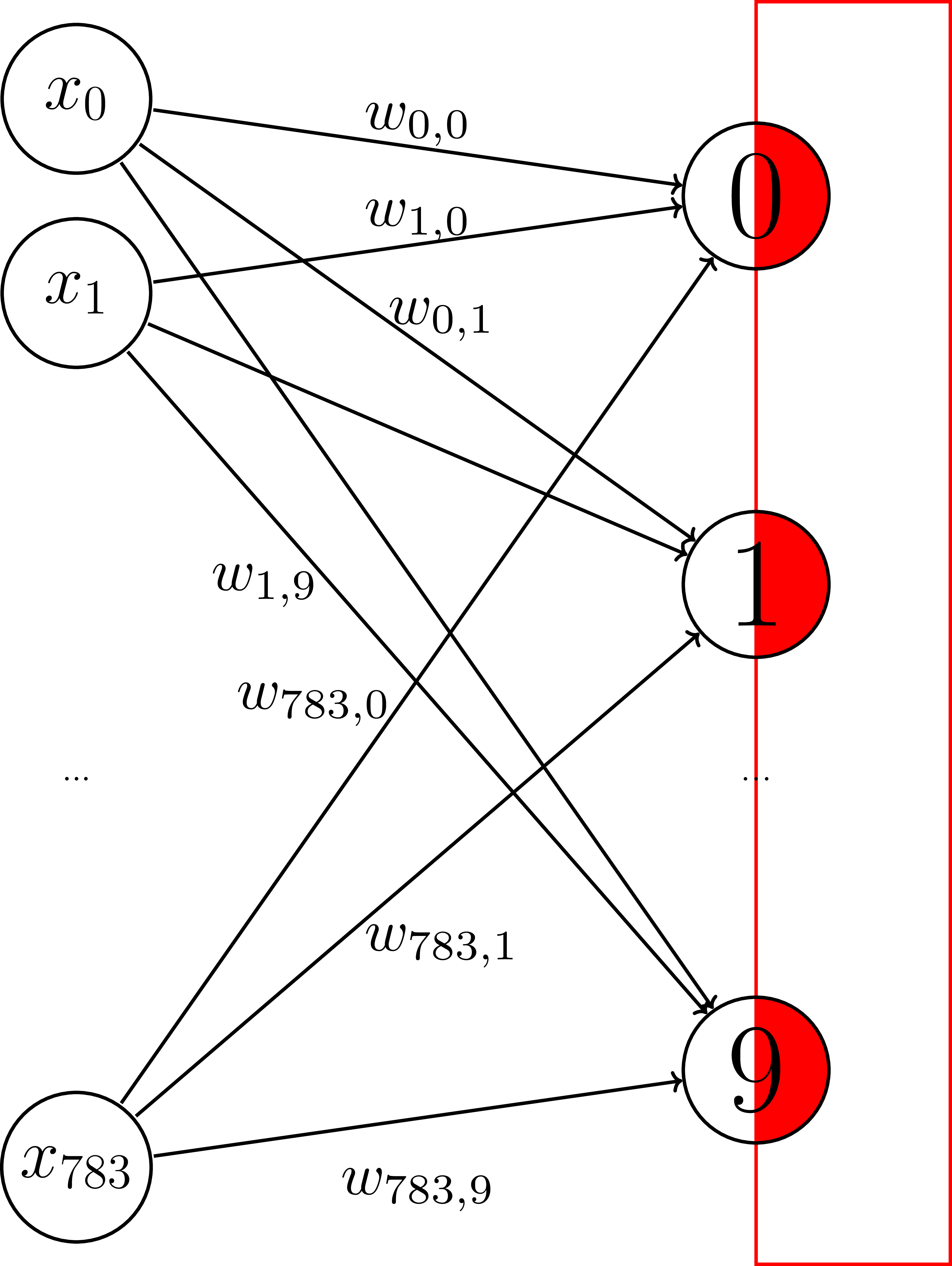
Placeholders
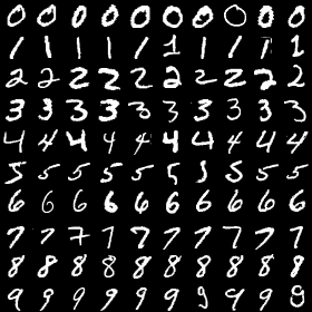
# X = vector length 784 (= 28 x 28 pixels)

# Y = one-hot vectors
# digit 0 = [1, 0, 0, 0, 0, 0, 0, 0, 0, 0]

X = tf.placeholder(tf.float32, [None, 28*28])
Y = tf.placeholder(tf.float32, [None, 10])
Variables
# Parameters/Variables
W = tf.get_variable("weights", [784, 10],
       initializer=tf.random_normal_initializer())
b = tf.get_variable("bias", [10],
       initializer=tf.constant_initializer(0))
Operations
Y_logits = tf.matmul(X, W) + b
Cost function
cost = tf.reduce_mean(
    tf.nn.softmax_cross_entropy_with_logits(
         logits=Y_logits, labels=Y))
Cost function
Cross Entropy$H(\hat{y}) = -\sum\limits_i y_i \log(\hat{y}_i)$
Optimization
learning_rate = 0.05
optimizer = tf.train.GradientDescentOptimizer
              (learning_rate).minimize(cost)
Training
with tf.Session() as sess:
    sess.run(tf.global_variables_initializer())

    for i in range(NUM_EPOCHS):
        for (X_batch, Y_batch) in get_minibatches(
                 X_train, Y_train, BATCH_SIZE):
            sess.run(optimizer,
                     feed_dict={X: X_batch,
                                Y: Y_batch})
Testing
predict = tf.argmax(Y_logits, 1)

with tf.Session() as sess:
    # training code from above

    predictions = sess.run(predict,
                    feed_dict={X: X_test})
    accuracy  = tf.reduce_mean(np.mean(
        np.argmax(Y_test, axis=1) == predictions)

>>> accuracy
0.925
Deficiencies of linear models
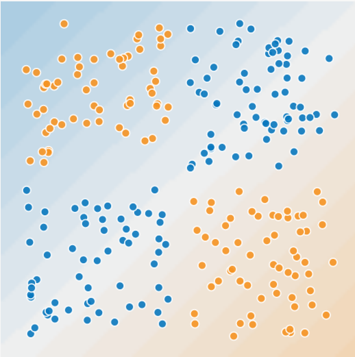
Image generated with playground.tensorflow.org
Deficiencies of linear models
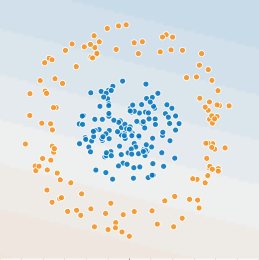
Image generated with playground.tensorflow.org
Let's go deeper!
Adding another layer
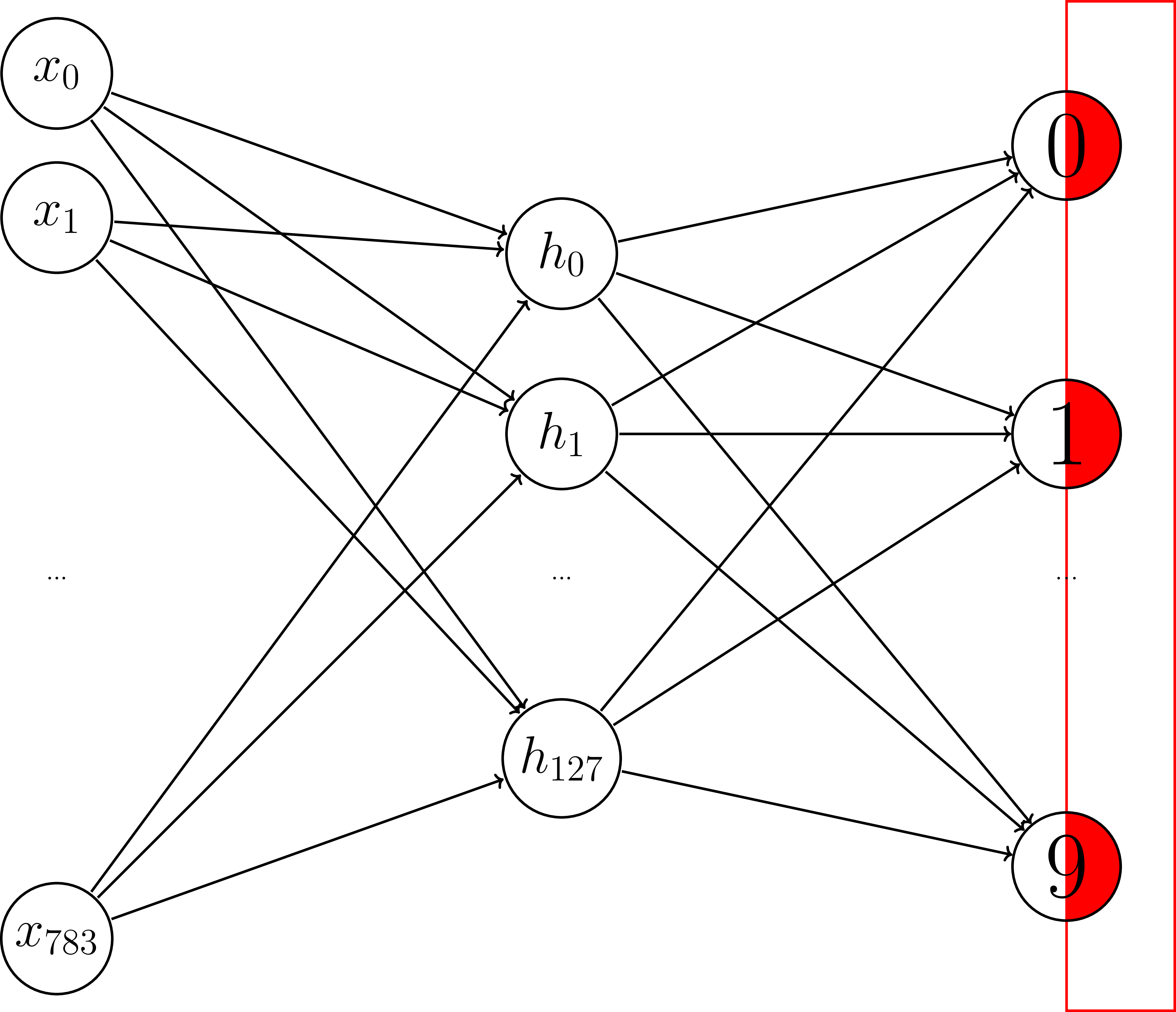
Adding another layer - Variables
HIDDEN_NODES = 128
W1 = tf.get_variable("weights1", [784, HIDDEN_NODES],
       initializer=tf.random_normal_initializer())
b1 = tf.get_variable("bias1", [HIDDEN_NODES],
       initializer=tf.constant_initializer(0))
W2 = tf.get_variable("weights2", [HIDDEN_NODES, 10],
      initializer=tf.random_normal_initializer())
b2 = tf.get_variable("bias2", [10],
      initializer=tf.constant_initializer(0))
Adding another layer - operations
hidden   = tf.matmul(X, W1) + b1
y_logits = tf.matmul(hidden, W2) + b2
Results
| # hidden layers | Train accuracy | Test accuracy |
| 0 | 93.0 | 92.5 |
| 1 | 89.2 | 88.8 |
Is Deep Learning just hype?
(Well, it's a little bit over-hyped...)
Problem
A linear transformation of a linear transformation is still a linear transformation!
We need to add non-linearity to the system.
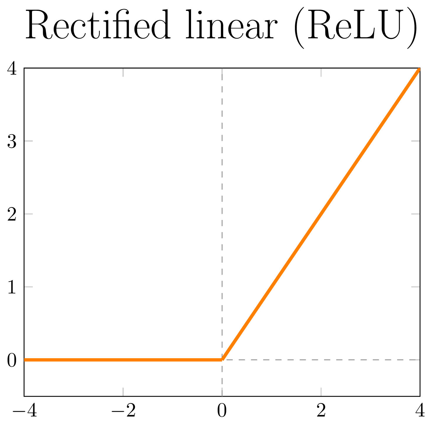
Adding non-linearity
Adding non-linearity
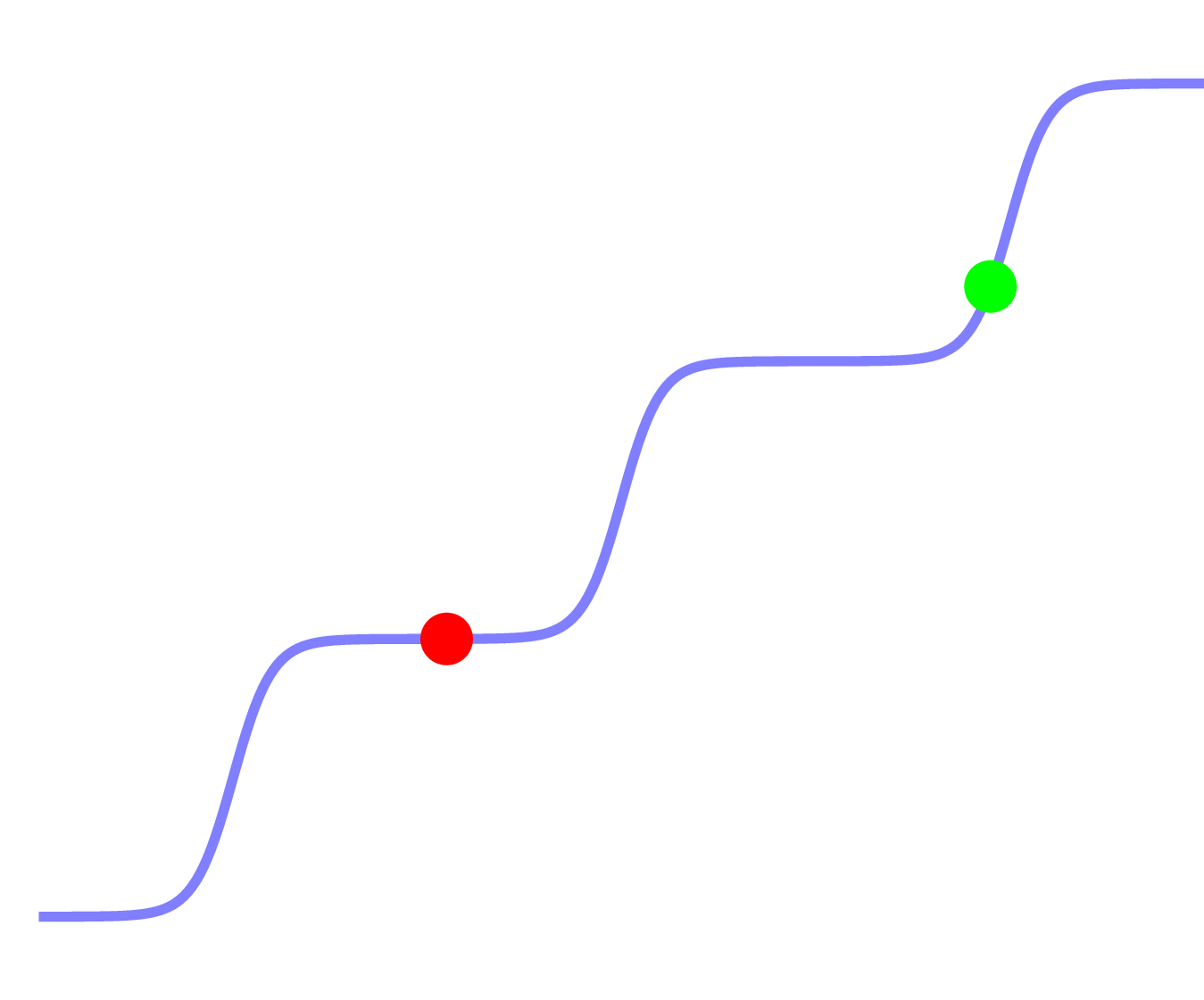
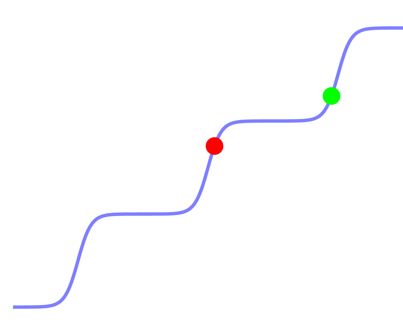
Non-linear activation functions
|
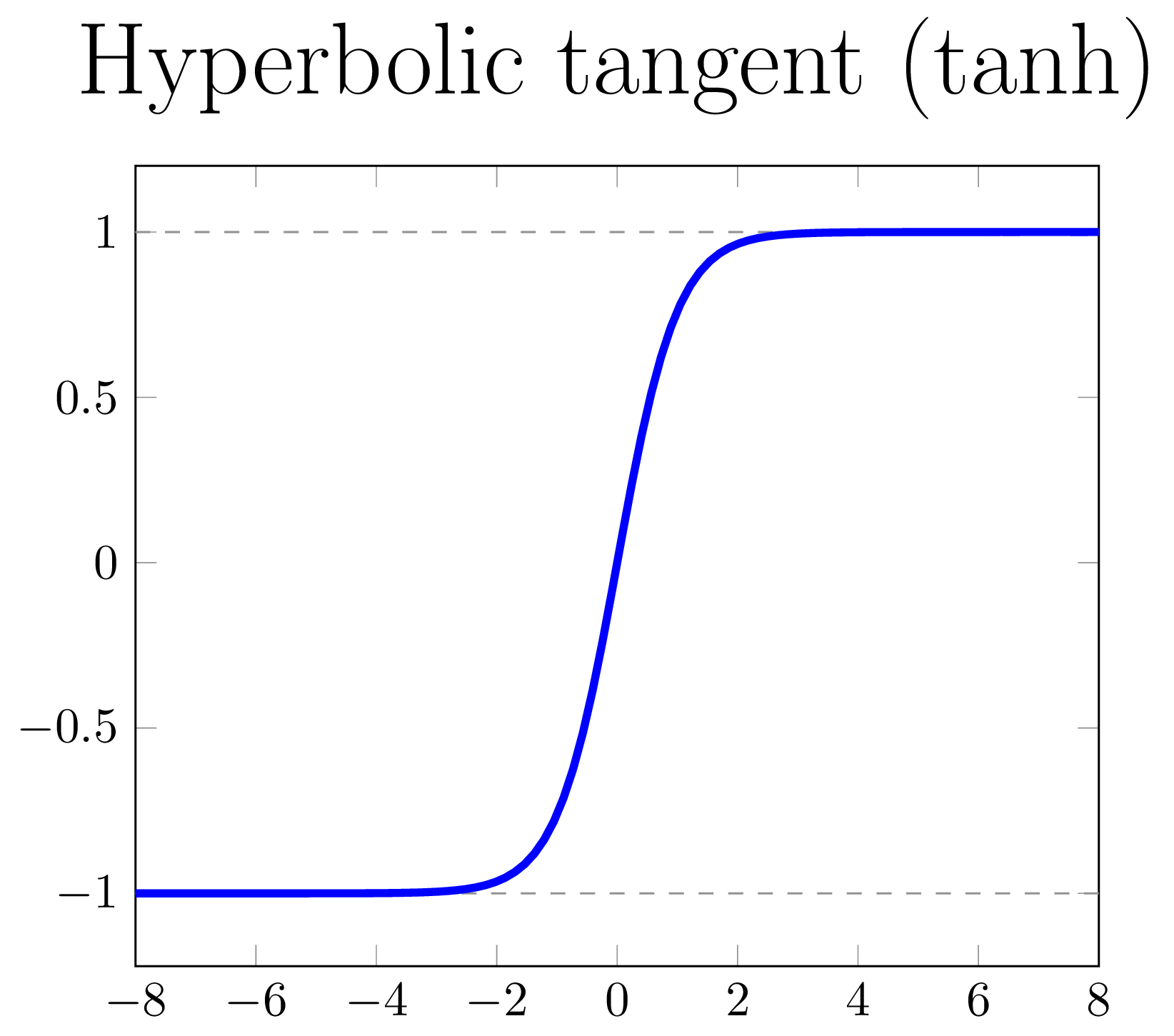
|
|
Adding non-linearity
Operations
hidden   = tf.nn.relu(tf.matmul(X, W1) + b1)
y_logits = tf.matmul(hidden, W2) + b2
Results
| # hidden layers | Train accuracy | Test accuracy |
| 0 | 93.0 | 92.5 |
| 1 | 97.9 | 95.2 |
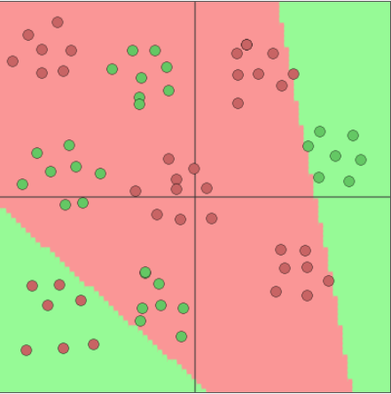
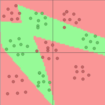
What the hidden layer bought us
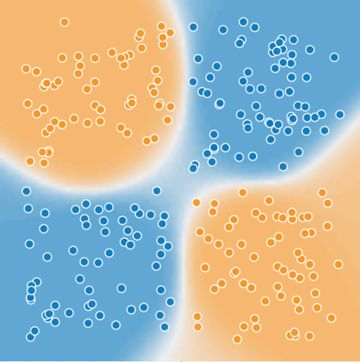
Image generated with playground.tensorflow.org
What the hidden layer bought us
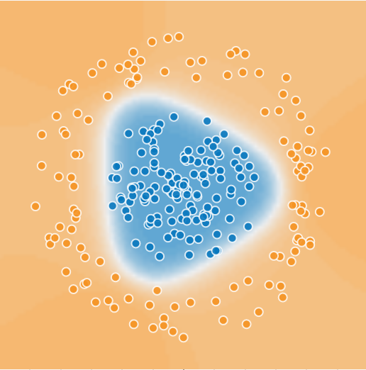
Image generated with playground.tensorflow.org
Adding hidden neurons
2 hidden neurons
Image generated with ConvNetJS by Andrej Karpathy
Adding hidden neurons
3 hidden neurons
Image generated with ConvNetJS by Andrej Karpathy
Adding hidden neurons
4 hidden neurons
Image generated with ConvNetJS by Andrej Karpathy
Adding hidden neurons

5 hidden neurons
Image generated with ConvNetJS by Andrej Karpathy
Adding hidden neurons
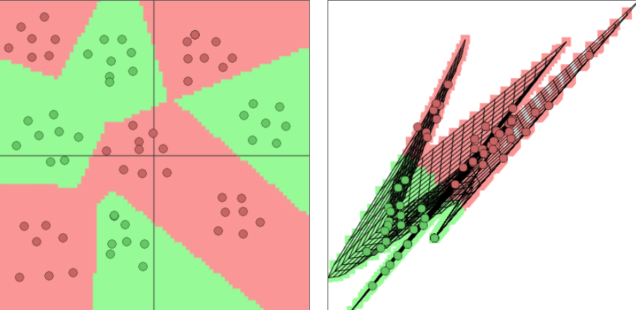
Image generated with ConvNetJS by Andrej Karpathy
Adding hidden neurons
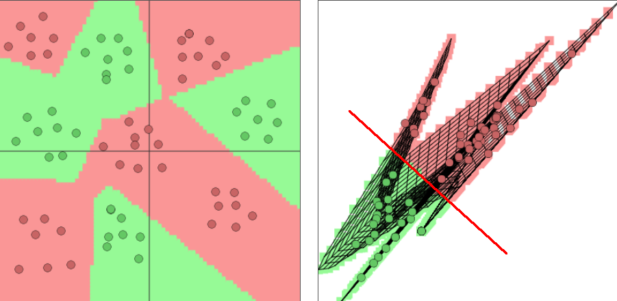
Image generated with ConvNetJS by Andrej Karpathy
Universal approximation theorem
A feedforward network with a single hidden layer containing a finite number of neurons can approximate (basically) any interesting functionAre we deep learning yet?
No!
Operations
hidden_1 = tf.nn.relu(tf.matmul(X, W1) + b1)
hidden_2 = tf.nn.relu(tf.matmul(hidden_1, W2) + b2)
y_logits = tf.matmul(hidden_2, W3) + b3
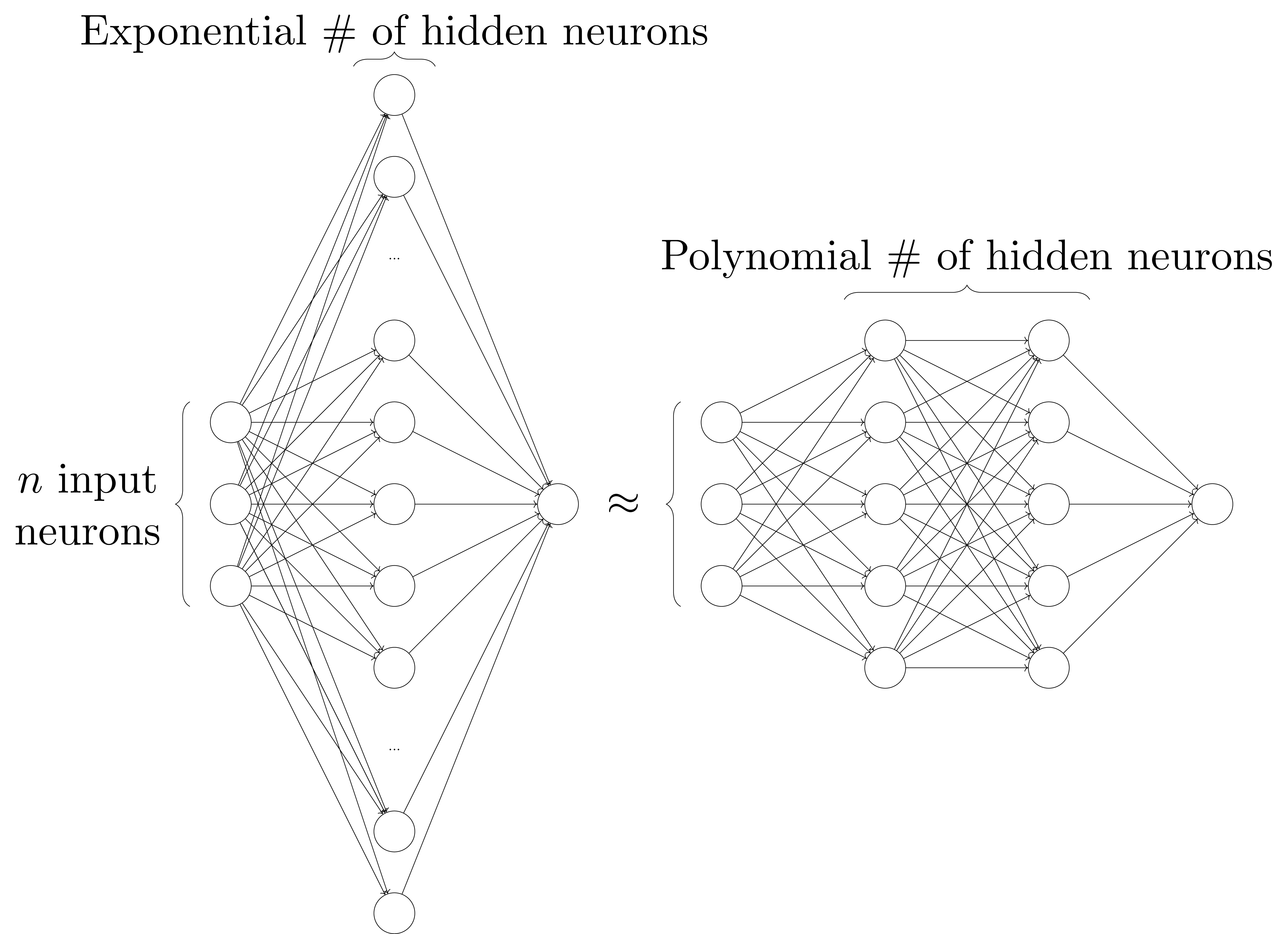
Why go deep?
3 reasons:- Deeper networks are more powerful
More powerful
Why go deep?
3 reasons:- Deeper networks are more powerful
- Narrower networks are less prone to overfitting
Overfitting
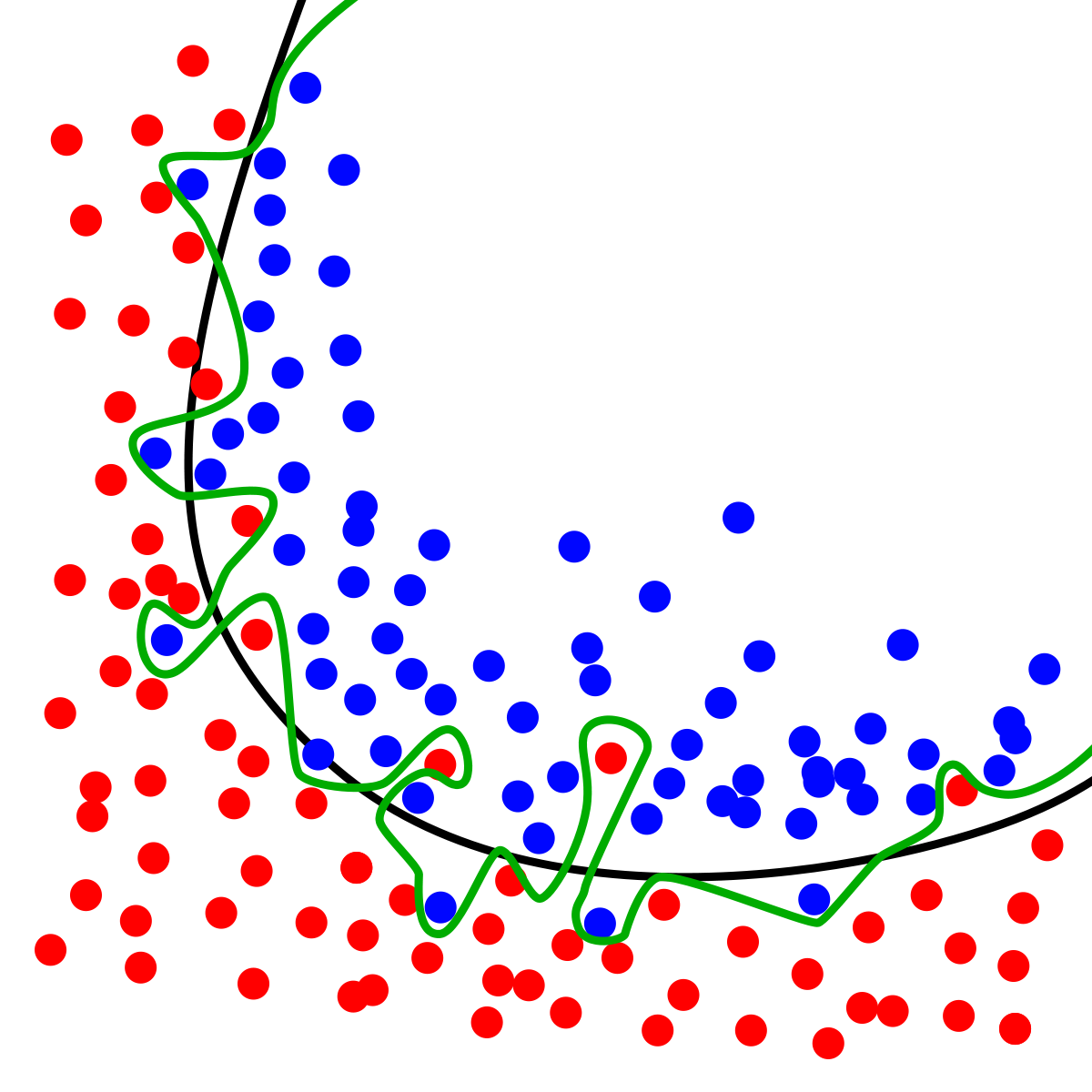
Less prone to overfitting
Why go deep?
3 reasons:- Deeper networks are more powerful
- Narrower networks are less prone to overfitting
- Deeper networks learn hierarchical feature representations
Learns hierarchical representations
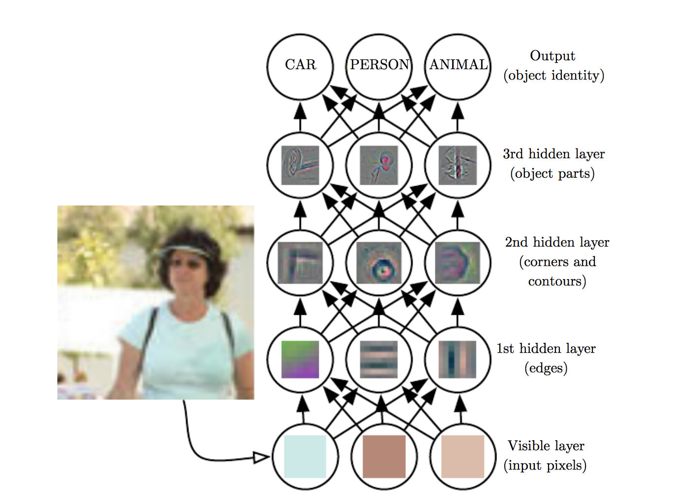
→ End-to-end learning
Image source: Goodfellow, Bengio, and Courville (2016) (The) Deep Learning (Book)
Why go deep?
3 reasons:- Deeper networks are more powerful
- Narrower networks are less prone to overfitting
- Deeper networks learn hierarchical feature representations
So let's go deeper!
Results
| # hidden layers | Train accuracy | Test accuracy |
| 0 | 93.0 | 92.5 |
| 1 | 97.9 | 95.2 |
| 2 | 98.0 | 94.2 |
Results
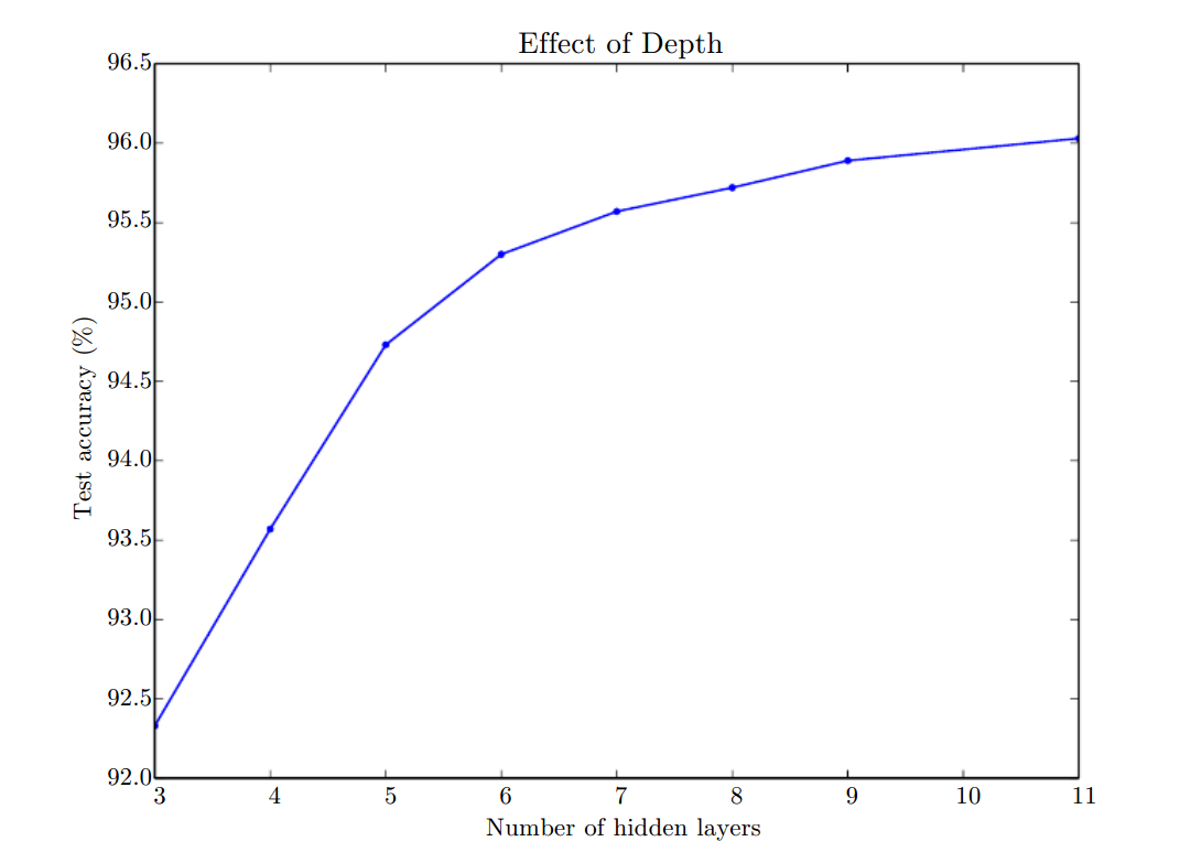
Image source: Goodfellow, Bengio, and Courville (2016) (The) Deep Learning (Book)
Overfitting

Regularization
Regularization
Put the brakes on the training data by enforcing constraints on weights.Regularization
L2 regularization: weights should be small.
$L = \sum{w_i^2}$L2 Regularization in TensorFlow
cost += REGULARIZATION_CONSTANT * \
          (tf.nn.l2_loss(W1) +
           tf.nn.l2_loss(W2) +
           tf.nn.l2_loss(W3))
Results
| Regularization | Train accuracy | Test accuracy |
| None | 95.5 | 92.9 |
| L2 | 95.1 | 95.1 |
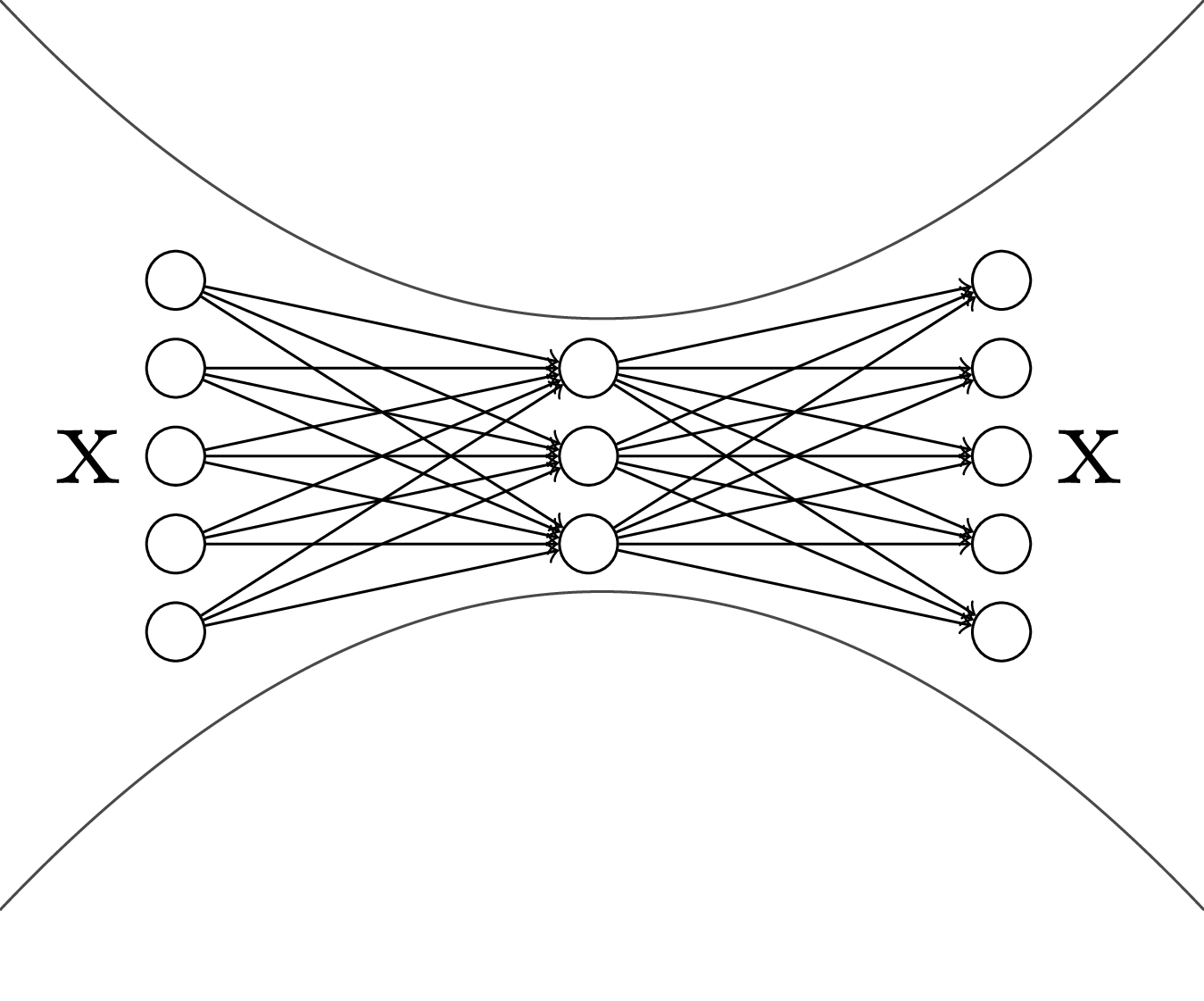
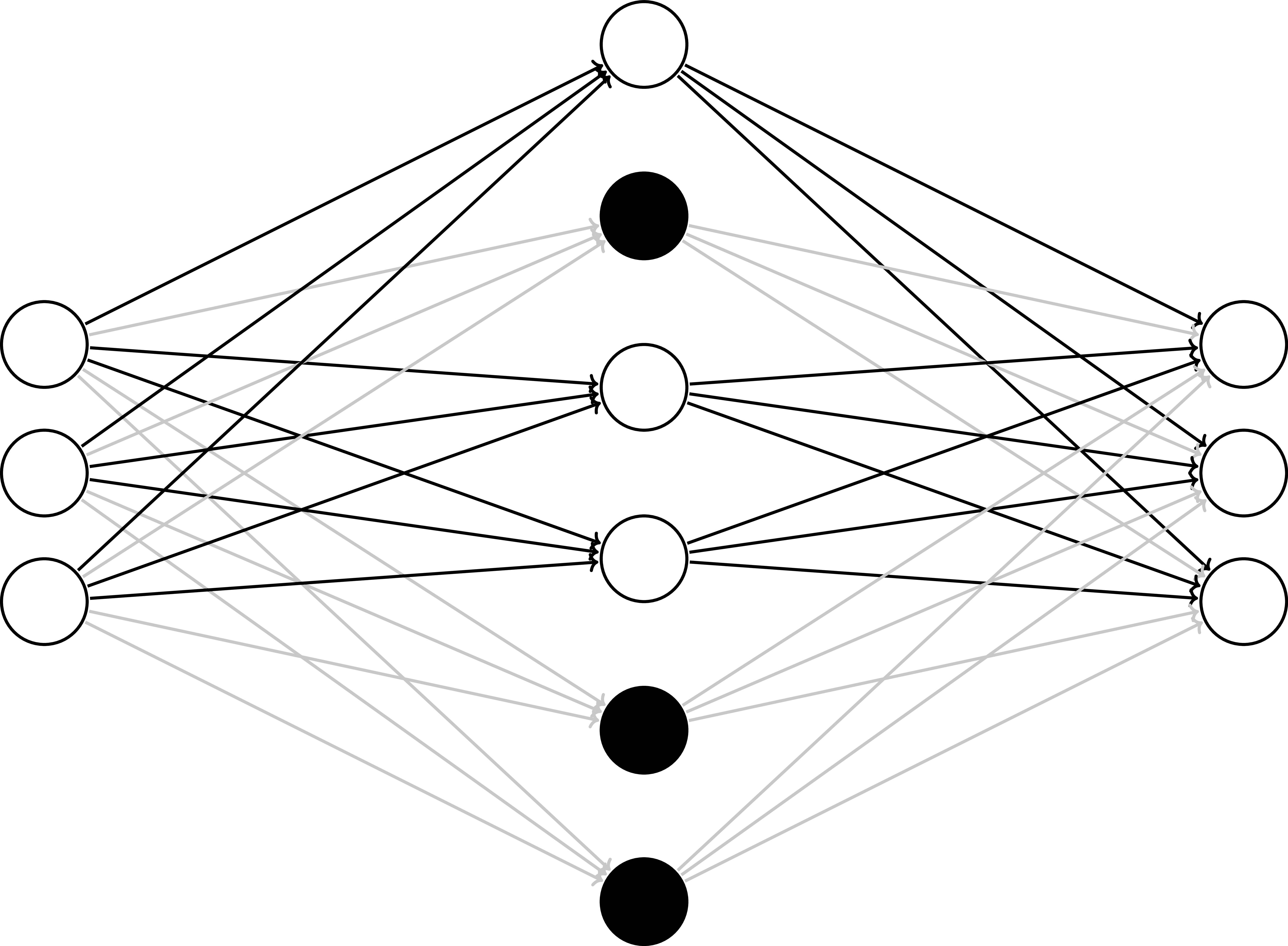
Dropout - Train
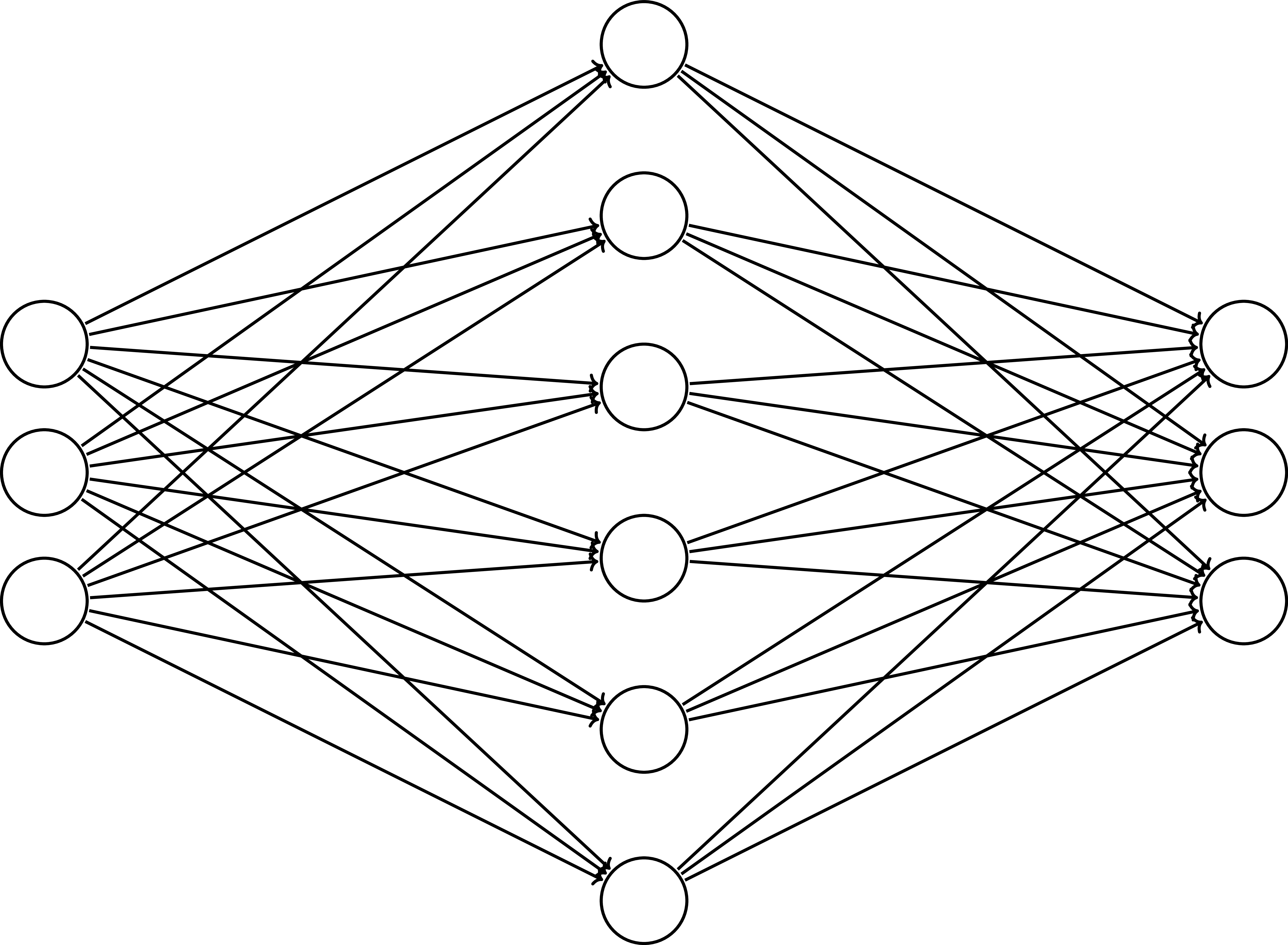
Dropout - Train
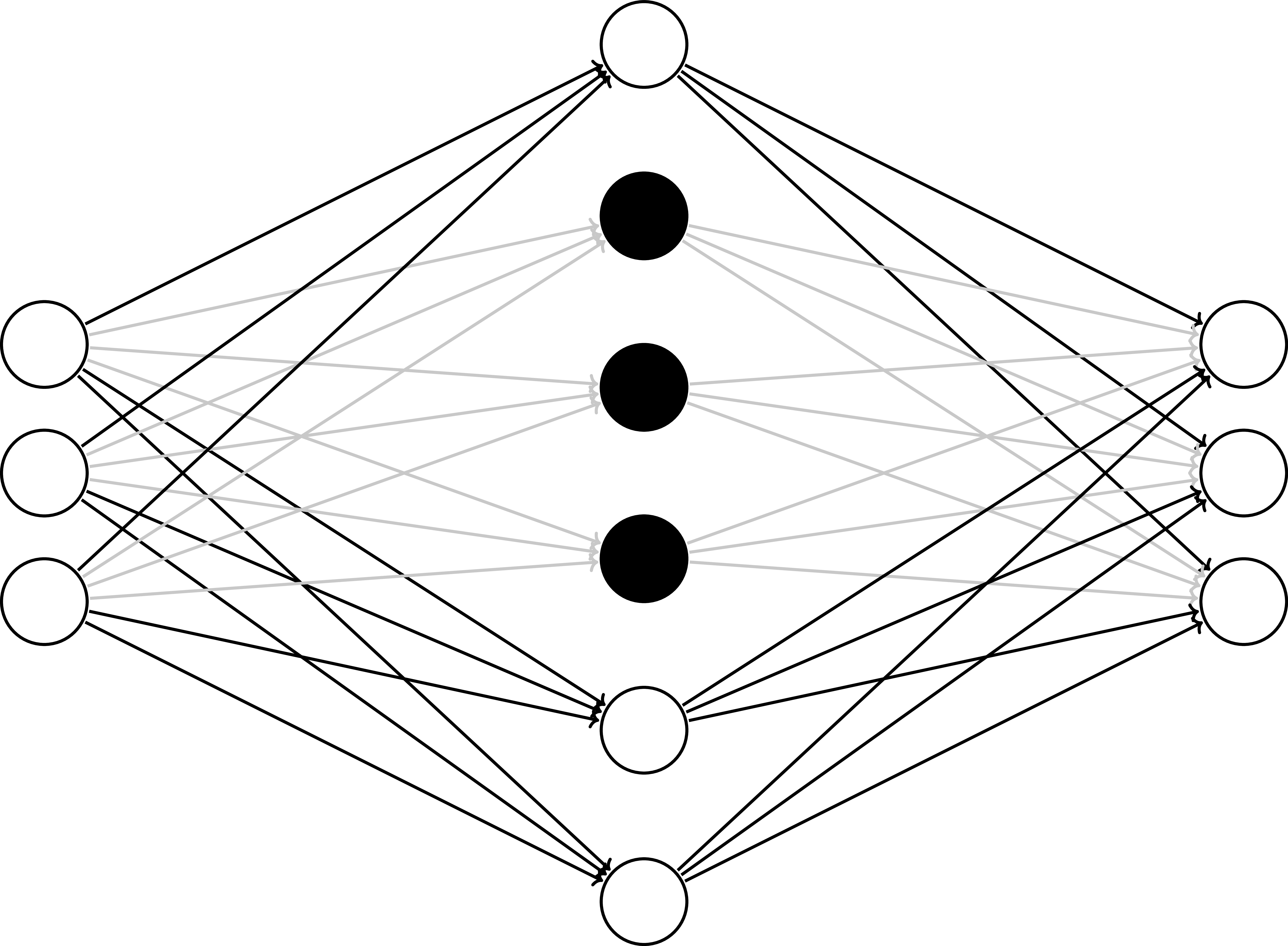
Dropout - Train
Dropout: why it works
- "Averaging" over several models
- Forces redundancy of useful features
- No conspiracies! Hidden neurons must be individually useful
Dropout - Test
Dropout - Train
Dropout in TensorFlow
# add a new placeholder
keep_prob = tf.placeholder(tf.float32)

# add a step to the model
hidden   = tf.nn.relu(tf.matmul(X, w0) + b0)
dropout  = tf.nn.dropout(hidden, keep_prob)
y_logits = tf.nn.relu(tf.matmul(dropout, w1) + b1)
Dropout in TensorFlow
with tf.Session() as sess:
    # ... init, then train:
    for _ in range(NUM_EPOCHS * 2):
        for (X_batch, Y_batch) in get_minibatches(
              X_train, Y_train, BATCH_SIZE):
            sess.run(optimizer,
                     feed_dict={
                         X: X_batch, Y: Y_batch,
                         keep_prob: 0.5
                     })

    # test
    sess.run(predict, feed_dict={X: X_test,
                            keep_prob: 1.0})
Results
| Regularization | Train accuracy | Test accuracy |
| None | 95.5 | 92.9 |
| L2 | 95.1 | 95.1 |
| Dropout | 93.3 | 93.1 |
Where to from here?
Ingredients
- Placeholders
- Model - Variables
- Model - Operations
- Cost function
- Optimization
- Train/Test
- Regularization
A guide to further exploration
- Placeholders
- Model - Variables
- Model - Operations
- Cost function
- Optimization
- Train/Test
- Regularization
A guide to further exploration
- Placeholders
- Model - Variables
- Model - Operations
- Cost function
- Optimization
- Train/Test
- Regularization
Model - Variables
# layers, # neurons / layer
Image source: Fjodor van Veen (2016) Neural Network Zoo
Model - Variables
- tf.random_normal_initializer
- tf.random_uniform_initializer
- tf.truncated_normal_initializer
- tf.constant_initializer
- tf.contrib.layers.xavier_initializer
Model - Operations
Activation functions: ReLU, tanh, leaky ReLU, Maxout...
Image source: Fjodor van Veen (2016) Neural Network Zoo
Model
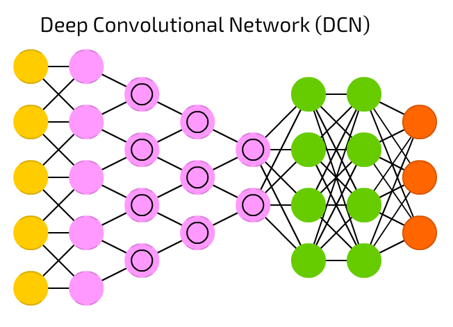
 Convolutional neural networks (images)
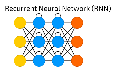
Recurrent neural networks (sequences & time series)
Image source: Fjodor van Veen (2016) Neural Network Zoo
Optimization
Try Adam
Image source: Alec Radford
Optimization & Regularization
- L1, L2 regularization
- Dropout
- Batch normalization
- Layer normalization
Other toolkits
- Torch (PyTorch)
- Caffe
- mxnet
- DyNet
- Many others...
Keras
$$ \begin{align*} \textrm{numpy} &: \textrm{scikit-learn} \\ &:: \\ \textrm{TensorFlow} &: \textrm{Keras} \end{align*} $$Keras
from keras.models import Sequential
model = Sequential()

model.add(Dense(input_dim=784, units=128, activation='relu'))
model.add(Dropout(0.5))
model.add(Dense(units=128, activation='relu'))
model.add(Dropout(0.5))
model.add(Dense(units=10, activation='softmax'))

model.compile(loss='categorical_crossentropy',
              optimizer=keras.optimizers.SGD(lr=0.05),
              metrics=['accuracy'])

model.fit(X_train, Y_train, epochs=100, batch_size=120)
model.evaluate(X_test, Y_test)
Final thoughts
- If you're familiar with traditional ML,
you can do deep learning! - But you'll need data. Lots of it.
- So try traditional ML first.
- Go forth and experiment!
- Thank you!
Slides: michelleful.github.io/PyCon2017