I built a linguistic street map of Singapore, with roads colour-coded by their linguistic origin!
Isn’t it pretty? :)
I talked about it at PyCon 2015, among other places. The slides and the video are both available. The code is up on Github in the form of some IPython notebooks, but I’ll be going through most of the essential steps in a series of blogposts, of which this is the first. So hang tight!
First, let me explain the motivation for making the map and the general shape of the project.
The push
If you’ve ever been in Singapore and glanced up at the street signs as you roamed, you’ll have noticed the considerable linguistic variety of Singapore road names. The reason, of course, is the multiplicity of races and ethnicities that immigrated to Singapore after the establishment of a port by the British in 1819.
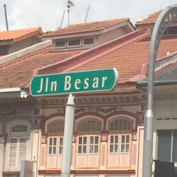
Joining the indigenous Malay population who gave their names to roads like Jalan Besar…
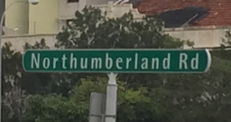
…were of course the British colonists (“Northumberland Road”)…
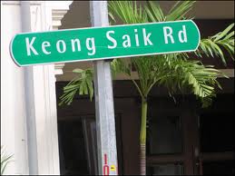
…people from the south of China speaking languages like Hokkien, Cantonese, and Teochew (“Keong Saik Road”), who eventually became the majority of the population…
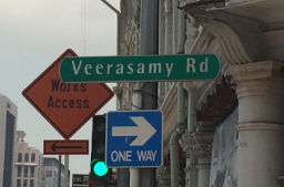
…and people from the south of India speaking languages like Tamil and Telugu (“Veerasamy Road”).
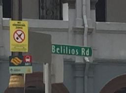
There were many other ethnicities besides - “Belilios Road” (Jewish), “Irrawaddy Road” (Burmese), etc…
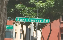
…And of course the usual “generic” sorts of names that describe either area landmarks like “Race Course Road” and “Stadium Link”, or other common nouns like “Sunrise Place” or “Cashew Road”.
While the road names are diverse, however, they’re far from evenly spread. For example, here’s a very British cluster of road names - Cambridge Road, Carlisle Road, Dorset Road, Owen Road, Norfolk Road, etc.
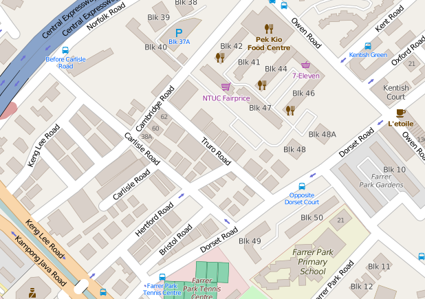 © Open Street Map contributors
And that’s just one of many.
I wanted an easy way to see how much clumpiness there was, and decided to visualise the clusters by plotting a map with roads colour-coded into the six categories I identified above (Malay, British, Chinese, Indian, Other Ethnicities, Generic). Something like this:
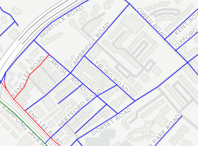 © Open Street Map contributors, © CartoDB
So all I needed was to get some road data (names, latitudes, longitudes), figure out which roads belonged to which categories, and plot that. Easy, right?
The plan
The first step was easy enough, at first glance. Singapore is pretty well-represented on OpenStreetMap, the crowd-sourced, openly licensed map of the world. But then I found that I needed to do all sorts of manipulation on the data. To my rescue came GeoPandas, an extension to the Pandas data analysis library that knows about geodata formats and can do all sorts of geographical manipulation and plotting. Using GeoPandas, I could filter and extract out the exact data I needed.
The next step was to assign categories to road names. I suppose I could have done this manually - there were only ~2000 unique names - but it would be tedious, and I wanted to try out scikit-learn, the Python machine learning library. Since I would be using supervised classification, which requires some labelled training data, I’d be doing some labelling anyway, but only a subset.
I decided to take an iterative approach to this: manually label 10% of the dataset, and use that as training data for an initial classifier. Use the classifier to train the next 10%, and hand-edit the incorrect labels. Now I’d have 20% of the dataset labelled, which I could use to train a better classifier, which I could use to label the next 10% of the data, etc.
I was asked at PyCon why I took this approach and I don’t think I gave a very thorough answer. It was really a mixture of four practical and psychological reasons:
- I’d only be addressing 10% of the data, or about 200 roads, at any one time. Much better than labelling a stack of 1000 roadnames!
- I’d need only 2 seconds or so to glance at a label and verify it was correct, and maybe 10 seconds to edit it (unless it needed further research, in which case it could take several minutes). Let’s suppose 30% of the roads came back labelled incorrectly. That’s about 15 minutes of work. Whereas labelling 200 roads from scratch would take twice as long.
- You know how they say the best way to get your question answered on the Internet is to post an incorrect hypothesis? Well, it was similar for me: when I saw that a road was labelled wrongly, I itched to correct it, whereas staring at a screen of road names with an empty column for labels was a great procrastination trigger.
- As the amount of labelled training data increased, the classifier gradually got better (although it peaked at about 50-60% of the data), so I had less and less work to do as time went on.
When you’re doing supervised classification, you need to come up with features that help to discriminate between the different categories. I tried a bunch of different features, and will talk about how to efficiently add them into your system using Pipelines (my favourite thing about scikit-learn)!
When everything was properly classified, I plotted the map in a couple of different ways. One was a quick data-exploration technique using GeoPandas’ own plotting feature, which I then turned into a webmap using a neat library called mplleaflet. The other was using CartoDB, which you see embedded above. I’ll talk about both these techniques, and alternatives to them.
The posts
So here’s the rough plan for the blogposts (if there’s a link it’s up):
- Getting data from OpenStreetMap and opening it in GeoPandas
- Manipulating geodata with GeoPandas
- Fuzzily cleaning data with fuzzywuzzy
- Building a baseline classifier in scikit-learn
- How to efficiently add features to a classifier using Pipelines and FeatureUnions
- Making the map in multiple ways
- What we've learned about Singapore roadnames!
Feel free to ask me any questions along this journey.